We now know how to project a signal onto other signals. We now need
to learn how to reconstruct a signal
![]() from its projections
onto
from its projections
onto ![]() different vectors
different vectors
![]() ,
,
![]() . This
will give us the inverse DFT operation (or the inverse of
whatever transform we are working with).
. This
will give us the inverse DFT operation (or the inverse of
whatever transform we are working with).
As a simple example, consider the projection of a signal
![]() onto the
rectilinear coordinate axes of
onto the
rectilinear coordinate axes of
![]() . The coordinates of the
projection onto the 0
th coordinate axis are simply
. The coordinates of the
projection onto the 0
th coordinate axis are simply
![]() .
The projection along coordinate axis
.
The projection along coordinate axis ![]() has coordinates
has coordinates
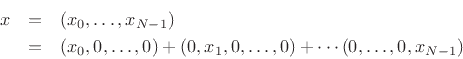
![]() , and so on. The original signal
, and so on. The original signal ![]() is then clearly
the vector sum of its projections onto the coordinate axes:
is then clearly
the vector sum of its projections onto the coordinate axes:
To make sure the previous paragraph is understood, let's look at the
details for the case ![]() . We want to project an arbitrary
two-sample signal
. We want to project an arbitrary
two-sample signal
![]() onto the coordinate axes in 2D. A
coordinate axis can be generated by multiplying any nonzero vector by
scalars. The horizontal axis can be represented by any vector of the
form
onto the coordinate axes in 2D. A
coordinate axis can be generated by multiplying any nonzero vector by
scalars. The horizontal axis can be represented by any vector of the
form
![]() ,
,
![]() while the vertical axis can be
represented by any vector of the form
while the vertical axis can be
represented by any vector of the form
![]() ,
,
![]() .
For maximum simplicity, let's choose
.
For maximum simplicity, let's choose
![\begin{eqnarray*}
\underline{e}_0 &\isdef & [1,0], \\
\underline{e}_1 &\isdef & [0,1].
\end{eqnarray*}](img888.png)
The projection of ![]() onto
onto
![]() is, by definition,
is, by definition,
![\begin{eqnarray*}
{\bf P}_{\underline{e}_0}(x) &\isdef & \frac{\left<x,\underline{e}_0\right>}{\Vert\underline{e}_0\Vert^2} \underline{e}_0\\ [5pt]
&=& \left<x,\underline{e}_0\right> \underline{e}_0
= \left<[x_0,x_1],[1,0]\right> \underline{e}_0
= (x_0 \cdot \overline{1} + x_1 \cdot \overline{0}) \underline{e}_0
= x_0 \underline{e}_0\\ [5pt]
&=& [x_0,0].
\end{eqnarray*}](img890.png)
Similarly, the projection of ![]() onto
onto
![]() is
is
![\begin{eqnarray*}
{\bf P}_{\underline{e}_1}(x) &\isdef & \frac{\left<x,\underline{e}_1\right>}{\Vert\underline{e}_1\Vert^2} \underline{e}_1\\ [5pt]
&=& \left<x,\underline{e}_1\right> \underline{e}_1
= \left<[x_0,x_1],[0,1]\right> \underline{e}_1
= (x_0 \cdot \overline{0} + x_1 \cdot \overline{1}) \underline{e}_1
= x_1 \underline{e}_1\\ [5pt]
&=& [0,x_1].
\end{eqnarray*}](img892.png)
The reconstruction of ![]() from its projections onto the coordinate
axes is then the vector sum of the projections:
from its projections onto the coordinate
axes is then the vector sum of the projections:
![$\displaystyle x= {\bf P}_{\underline{e}_0}(x) + {\bf P}_{\underline{e}_1}(x) = x_0 \underline{e}_0 + x_1 \underline{e}_1
\isdef x_0 \cdot [1,0] + x_1 \cdot [0,1] = (x_0,x_1)
$](img893.png)
The projection of a vector onto its coordinate axes is in some sense
trivial because the very meaning of the coordinates is that they are
scalars ![]() to be applied to the coordinate vectors
to be applied to the coordinate vectors
![]() in
order to form an arbitrary vector
in
order to form an arbitrary vector
![]() as a linear combination
of the coordinate vectors:
as a linear combination
of the coordinate vectors:
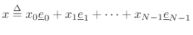
Note that the coordinate vectors are orthogonal. Since they are also unit length,