- ...
email1.1
- jos at ccrma
.
.
.
.
.
.
.
.
.
.
.
.
.
.
.
.
.
.
.
.
.
.
.
.
.
.
.
.
.
.
- ... analysis.2.1
- Testing a filter by
sweeping an input sinusoid through a range of frequencies is often
used in practice, especially when there might be some distortion that
also needs to be measured. There are particular advantages to using
exponentially swept sine-wave analysis
[24], in which
the sinusoidal frequency increases exponentially with respect to time.
(The technique is sometimes also referred to as log-swept
sine-wave analysis.) Swept-sine analysis can be viewed as a
descendant of time-delay spectrometry.
.
.
.
.
.
.
.
.
.
.
.
.
.
.
.
.
.
.
.
.
.
.
.
.
.
.
.
.
.
.
- ...real2.2
- We may define a real filter as one whose
output signal is real whenever its input signal is real.
.
.
.
.
.
.
.
.
.
.
.
.
.
.
.
.
.
.
.
.
.
.
.
.
.
.
.
.
.
.
- ...
sinusoid|textbf.2.3
- Some authors refer to
 as a
complex exponential, but it is useful to reserve that term for
signals of the form
as a
complex exponential, but it is useful to reserve that term for
signals of the form
 , where
  . That is,
complex exponentials are more generally allowed to have a
non-constant exponential amplitude envelope.
Note that all complex exponentials can be generated from two complex
numbers,
. That is,
complex exponentials are more generally allowed to have a
non-constant exponential amplitude envelope.
Note that all complex exponentials can be generated from two complex
numbers,
 and
and
 , viz.,
 . This topic is explored further in [84].
.
.
.
.
.
.
.
.
.
.
.
.
.
.
.
.
.
.
.
.
.
.
.
.
.
.
.
.
.
.
- ...
Octave,3.1
- Users of Matlab will also need the Signal Processing
Toolbox, which is available for an additional charge. Users of
Octave will also need the free ``Octave Forge'' collection, which
contains functions corresponding to the Signal Processing Toolbox.
.
.
.
.
.
.
.
.
.
.
.
.
.
.
.
.
.
.
.
.
.
.
.
.
.
.
.
.
.
.
- ...
language.3.2
- In an effort to improve the matlab language, Octave
does not maintain 100% compatibility with Matlab. See
http://octave.sf.net/compatibility.html
for details.
.
.
.
.
.
.
.
.
.
.
.
.
.
.
.
.
.
.
.
.
.
.
.
.
.
.
.
.
.
.
- ...filter3.3
- Say help filter in Matlab or Octave
to view the documentation. In Matlab, you can also say doc
filter to view more detailed documentation in a Web browser.
.
.
.
.
.
.
.
.
.
.
.
.
.
.
.
.
.
.
.
.
.
.
.
.
.
.
.
.
.
.
- ... filter:3.4
- These adjectives will be
defined precisely in Chapters 4 and 5.
.
.
.
.
.
.
.
.
.
.
.
.
.
.
.
.
.
.
.
.
.
.
.
.
.
.
.
.
.
.
- ...
1.3.5
- As we will learn in §5.1, A(1) is the
coefficient of the current output sample, which is always
normalized to 1. The actual feedback coefficients are
 .
.
.
.
.
.
.
.
.
.
.
.
.
.
.
.
.
.
.
.
.
.
.
.
.
.
.
.
.
.
.
.
- ...,3.6
- The notation
 denotes the half-open interval--the set of all real
numbers between
denotes the half-open interval--the set of all real
numbers between  and
and  , including
but not
.
, including
but not
.
.
.
.
.
.
.
.
.
.
.
.
.
.
.
.
.
.
.
.
.
.
.
.
.
.
.
.
.
.
.
- ... execution.3.7
- As a fine point, the fastest known FFT for
power-of-2 lengths is the split-radix FFT--a hybrid of the
radix-2 and radix-4 cases. See
http://cnx.org/content/m12031/latest/
for more details.
.
.
.
.
.
.
.
.
.
.
.
.
.
.
.
.
.
.
.
.
.
.
.
.
.
.
.
.
.
.
- ...MDFT.3.8
- http://ccrma.stanford.edu/~jos/mdft/
.
.
.
.
.
.
.
.
.
.
.
.
.
.
.
.
.
.
.
.
.
.
.
.
.
.
.
.
.
.
- ...
matlab4.1
- The term ``matlab'' (uncapitalized) will refer here to
either Matlab or Octave [82]. Code described
as ``matlab'' should run in either environment without modification.
.
.
.
.
.
.
.
.
.
.
.
.
.
.
.
.
.
.
.
.
.
.
.
.
.
.
.
.
.
.
- ... completeness.4.2
- Most plots in
this book are optimized for Matlab. Octave uses
gnuplot which is quite different from Matlab's
handle-oriented graphics. In Octave, the plots will typically be
visible, but the titles and axis labels may be incorrect due to the
different semantics associated with statement ordering in the two
cases.
.
.
.
.
.
.
.
.
.
.
.
.
.
.
.
.
.
.
.
.
.
.
.
.
.
.
.
.
.
.
- ... frequency:4.3
- As always,
radian frequency
 is related to frequency
  in Hz by the
relation
in Hz by the
relation
 . Also as always in this book, the sampling
rate is denoted by
. Also as always in this book, the sampling
rate is denoted by  . Since the frequency axis for digital
signals goes from
. Since the frequency axis for digital
signals goes from  to
to  (non-inclusive), we have
 , where
  denotes a half-open interval. Since the
frequency
denotes a half-open interval. Since the
frequency
 is usually rejected in applications, it is more
practical to take
is usually rejected in applications, it is more
practical to take
 .
.
.
.
.
.
.
.
.
.
.
.
.
.
.
.
.
.
.
.
.
.
.
.
.
.
.
.
.
.
.
.
- ...
``echo''.4.4
- The minimum perceivable delay in audio work depends
very much on how the filter is being used and also on what signals are
being filtered. A few milliseconds of delay is usually not
perceivable in the monaural case. Note, however, that delay
perception is a function of frequency. One rule of thumb is that, to
be perceived as instantaneous, a filter's delay should be kept below a
few cycles at each frequency. A near-worst-case test signal for
monaural filter-delay perception is an impulse (pure click). (A
worst-case test would require some weighting vs. frequency.) Delay
distortion is less noticeable if all frequencies in a signal are
delayed by the same amount of time, since that preserves the original
waveshape exactly and delays it as a whole. Otherwise transient
smearing occurs, and the ear is fairly sensitive to onset synchrony
across different frequency bands.
.
.
.
.
.
.
.
.
.
.
.
.
.
.
.
.
.
.
.
.
.
.
.
.
.
.
.
.
.
.
- ...5.1
- One might argue that
nonlinear filters must be considered a special case of time-varying
filters, because any variation in the filter coefficients must occur
over time, and in the nonlinear case, this variation simply happens to
occur in a manner that depends on the input signal sample values.
However, since a constant signal (dc) does not vary over time, a
nonlinear filter may also be time-invariant. As we will see in
this chapter, the key test for nonlinearity is whether the filter
coefficients change as a function of the input signal.
A linear time-varying filter, on the other hand, must exhibit
the same coefficient variation over time for all input
signals.
.
.
.
.
.
.
.
.
.
.
.
.
.
.
.
.
.
.
.
.
.
.
.
.
.
.
.
.
.
.
- ... space5.2
- A set of vectors
 (or
(or
 )
is said to form a vector space if
)
is said to form a vector space if
 and
and
 for all
 ,
,
 , and for all scalars
 (or
(or
 ) [84,73].
.
.
.
.
.
.
.
.
.
.
.
.
.
.
.
.
.
.
.
.
.
.
.
.
.
.
.
.
.
.
- ... purposes.5.3
-
For more about the mathematics of linear vector spaces, look into
linear algebra [58] (which covers finite-dimensional
linear vector spaces) and/or operator theory
[56] (which treats the infinite-dimensional case).
The mathematical treatments used in this book will be closer to
complex analysis [14,43], but with some linear
algebra concepts popping up from time to time, especially in the
context of matlab examples. (The name ``matlab'' derives from ``matrix
laboratory,'' and it was originally written by Cleve Moler to be an
interactive desk-calculator front end for a library of numerical
linear algebra subroutines (LINPACK and EISPACK).
As a result, matlab syntax is designed to follow linear algebra
notation as closely as possible.)
.
.
.
.
.
.
.
.
.
.
.
.
.
.
.
.
.
.
.
.
.
.
.
.
.
.
.
.
.
.
- ... domain.6.1
- The term ``difference
equation'' is a discrete-time counterpart to the term ``differential
equation'' in continuous time. LTI difference equations in discrete
time correspond to linear differential equations with
constant coefficients in continuous time. The subject of
finite differences is devoted to ``discretizing'' differential
equations to obtain difference equations [96,3].
.
.
.
.
.
.
.
.
.
.
.
.
.
.
.
.
.
.
.
.
.
.
.
.
.
.
.
.
.
.
- ...
scheme|textbf.6.2
- The term ``explicit'' in this context means that the
output
 at time
  can be computed using only past
output samples
can be computed using only past
output samples  ,
,  , etc. When solving partial
differential equations numerically on a grid in 2 or more dimensions,
it is possible to derive finite difference schemes which cannot be
computed recursively, and these are termed implicit finite
difference schemes [96,3]. Implicit schemes can
often be converted to explicit schemes by a change of coordinates
(e.g., to modal coordinates [86]).
, etc. When solving partial
differential equations numerically on a grid in 2 or more dimensions,
it is possible to derive finite difference schemes which cannot be
computed recursively, and these are termed implicit finite
difference schemes [96,3]. Implicit schemes can
often be converted to explicit schemes by a change of coordinates
(e.g., to modal coordinates [86]).
.
.
.
.
.
.
.
.
.
.
.
.
.
.
.
.
.
.
.
.
.
.
.
.
.
.
.
.
.
.
- ... filter.6.3
- Instead of defining
the impulse response as the response of the filter to
 , a
unit-amplitude impulse arriving at time zero, we could equally well
choose our ``standard impulse'' to be
, a
unit-amplitude impulse arriving at time zero, we could equally well
choose our ``standard impulse'' to be
 , an
amplitude-
, an
amplitude- impulse arriving at time
  . However, setting
 and
and  makes the math simpler to write, as we will see.
.
.
.
.
.
.
.
.
.
.
.
.
.
.
.
.
.
.
.
.
.
.
.
.
.
.
.
.
.
.
- ...MDFT6.4
- http://ccrma.stanford.edu/~jos/mdft/Convolution.html
.
.
.
.
.
.
.
.
.
.
.
.
.
.
.
.
.
.
.
.
.
.
.
.
.
.
.
.
.
.
- ...MDFT6.5
- http://ccrma.stanford.edu/~jos/mdft/
.
.
.
.
.
.
.
.
.
.
.
.
.
.
.
.
.
.
.
.
.
.
.
.
.
.
.
.
.
.
- ... causal,7.1
- In a causal filter (§5.3),
each output sample is computed using only current and past input
samples--no future samples. A causal signal is similarly
zero before time zero (
 ). An LTI filter is
causal if and only if its impulse response is a causal signal.
). An LTI filter is
causal if and only if its impulse response is a causal signal.
.
.
.
.
.
.
.
.
.
.
.
.
.
.
.
.
.
.
.
.
.
.
.
.
.
.
.
.
.
.
- ...
points7.2
- When
 is a filter transfer function (i.e.,
  is a filter impulse response), these singularities are called
poles of the transfer function, as will be defined in
§6.6 below. Analogously, one can speak of ``poles'' in the
z transform of a signal containing exponential components of the form
is a filter impulse response), these singularities are called
poles of the transfer function, as will be defined in
§6.6 below. Analogously, one can speak of ``poles'' in the
z transform of a signal containing exponential components of the form
 .
.
.
.
.
.
.
.
.
.
.
.
.
.
.
.
.
.
.
.
.
.
.
.
.
.
.
.
.
.
.
.
- ...
follows:7.3
- Each `
' in these equations should be interpreted
as `
 '.
'.
.
.
.
.
.
.
.
.
.
.
.
.
.
.
.
.
.
.
.
.
.
.
.
.
.
.
.
.
.
.
- ... terms,7.4
- By the fundamental theorem of
algebra, a polynomial
 of any degree can be completely factored
as a product of first-order polynomials, where the zeros may be complex.
of any degree can be completely factored
as a product of first-order polynomials, where the zeros may be complex.
.
.
.
.
.
.
.
.
.
.
.
.
.
.
.
.
.
.
.
.
.
.
.
.
.
.
.
.
.
.
- ...residuez7.5
- Matlab Signal Processing
Toolbox or Octave Forge collection--see also
§J.5 (p.
![[*]](../icons/crossref.png) ).
).
.
.
.
.
.
.
.
.
.
.
.
.
.
.
.
.
.
.
.
.
.
.
.
.
.
.
.
.
.
.
- ...biquads.7.6
- A biquad is simply a second-order filter section--see
§B.1.6 for details.
.
.
.
.
.
.
.
.
.
.
.
.
.
.
.
.
.
.
.
.
.
.
.
.
.
.
.
.
.
.
- ...
function|textbf.7.7
- The case
 is called a proper transfer
function, and
is called a proper transfer
function, and  is termed improper.
.
.
.
.
.
.
.
.
.
.
.
.
.
.
.
.
.
.
.
.
.
.
.
.
.
.
.
.
.
.
- ... filter7.8
- In physical models, such a superposition of
identical resonances is often called degeneracy
[86].
.
.
.
.
.
.
.
.
.
.
.
.
.
.
.
.
.
.
.
.
.
.
.
.
.
.
.
.
.
.
- ... coefficients7.9
- We would like to use the
term residue here instead of coefficient, but strictly
speaking the coefficient
 in the pole-term
 is
the residue of the pole
is
the residue of the pole  only when
  (multiplicity one);
when
is any integer other than 1, the residue is zero (see any
book on complex analysis and/or Cauchy's Residue Theorem). For
(multiplicity one);
when
is any integer other than 1, the residue is zero (see any
book on complex analysis and/or Cauchy's Residue Theorem). For  ,
we will try to remember to call
the ``
th coefficient'' of the
pole
.
,
we will try to remember to call
the ``
th coefficient'' of the
pole
.
.
.
.
.
.
.
.
.
.
.
.
.
.
.
.
.
.
.
.
.
.
.
.
.
.
.
.
.
.
.
- ...
on:7.10
-
These closed-form sums were quickly computed using the
free symbolic mathematics program called maxima running under
Linux, specifically by typing
factor(ev(sum(m+1,m,0,n),simpsum)); followed by
factor(ev(sum(%,n,0,m),simpsum));.
.
.
.
.
.
.
.
.
.
.
.
.
.
.
.
.
.
.
.
.
.
.
.
.
.
.
.
.
.
.
- ...B2.7.11
- Since convolution is
commutative,
either operand to a convolution can be interpreted as the filter
impulse-response while the other is interpreted as the input
signal. However, in the matlab filter function, the operand
designated as the input signal (3rd argument) determines the length to
which the output signal is truncated.
.
.
.
.
.
.
.
.
.
.
.
.
.
.
.
.
.
.
.
.
.
.
.
.
.
.
.
.
.
.
- ...MDFT.8.1
- Some elementary
review regarding signals and spectra is given in Appendix A.
.
.
.
.
.
.
.
.
.
.
.
.
.
.
.
.
.
.
.
.
.
.
.
.
.
.
.
.
.
.
- ... ripple8.2
- A passband may be defined as any frequency band that the filter
is trying to ``pass''--i.e., not trying to suppress. For example, in
a lowpass filter with cut-off frequency
 , the passband is
the interval
, the passband is
the interval
![$ [-\omega_c,\omega_c]$](img878.png) . A lowpass filter typically also
has a stopband that the filter is designed to suppress.
For practical realizability, there should be a transition band
between a passband and stopband. In some simple filters, such as
Butterworth filters introduced in §7.6.4 below, there are
passbands but no stopbands; instead, the stopband is replaced by a
roll-off, typically specifiable in dB/octave. (The rolloff
region can be viewed as a transition band between a passband and a
``stop point'' such as some number of zeros at
. A lowpass filter typically also
has a stopband that the filter is designed to suppress.
For practical realizability, there should be a transition band
between a passband and stopband. In some simple filters, such as
Butterworth filters introduced in §7.6.4 below, there are
passbands but no stopbands; instead, the stopband is replaced by a
roll-off, typically specifiable in dB/octave. (The rolloff
region can be viewed as a transition band between a passband and a
``stop point'' such as some number of zeros at
 for
lowpass filters, or
for
lowpass filters, or  for highpass filters. Within a
passband or stopband, the amplitude response may exhibit
ripple, that is, it may oscillate about the desired band gain,
as discussed further in §7.6.4 below. A ripple
specification sets a maximum deviation limit on the ripple.
for highpass filters. Within a
passband or stopband, the amplitude response may exhibit
ripple, that is, it may oscillate about the desired band gain,
as discussed further in §7.6.4 below. A ripple
specification sets a maximum deviation limit on the ripple.
.
.
.
.
.
.
.
.
.
.
.
.
.
.
.
.
.
.
.
.
.
.
.
.
.
.
.
.
.
.
- ...freqzDemoTwo.8.3
- The ``multiplot''
created by the plotfr utility (§J.4) cannot be
saved to disk in Octave, although it looks fine on screen. In Matlab,
there is no problem saving multiplots to disk.
.
.
.
.
.
.
.
.
.
.
.
.
.
.
.
.
.
.
.
.
.
.
.
.
.
.
.
.
.
.
- ....8.4
- The quantity
 is known as the
para-Hermitian conjugate of the polynomial
. It coincides
with the ordinary complex conjugate along the unit
circle, while elsewhere in the
is known as the
para-Hermitian conjugate of the polynomial
. It coincides
with the ordinary complex conjugate along the unit
circle, while elsewhere in the  -plane,
is replaced by
-plane,
is replaced by  and
only the coefficients of
are conjugated. A mathematical feature
of the para-Hermitian conjugate is that
is an
analytic function of
while
and
only the coefficients of
are conjugated. A mathematical feature
of the para-Hermitian conjugate is that
is an
analytic function of
while
 is not.
.
.
.
.
.
.
.
.
.
.
.
.
.
.
.
.
.
.
.
.
.
.
.
.
.
.
.
.
.
.
- ....9.1
- See
§6.2 and
§8.7 for related discussion.
.
.
.
.
.
.
.
.
.
.
.
.
.
.
.
.
.
.
.
.
.
.
.
.
.
.
.
.
.
.
- ... grow.9.2
- As discussed in §6.8.5, the
impulse response of a repeated pole of multiplicity
 at a
point on the unit circle may grow with amplitude envelope proportional
to
at a
point on the unit circle may grow with amplitude envelope proportional
to  .
.
.
.
.
.
.
.
.
.
.
.
.
.
.
.
.
.
.
.
.
.
.
.
.
.
.
.
.
.
.
.
- ...PASP.9.3
-
See, e.g., http://ccrma.stanford.edu/~jos/pasp/Passive_Reflectances.html
.
.
.
.
.
.
.
.
.
.
.
.
.
.
.
.
.
.
.
.
.
.
.
.
.
.
.
.
.
.
.
- ...
time-constant|textbf9.4
- Decay time constants were introduced in Book I
[84] of this series (``Exponentials''). The time
constant
 is formally defined for exponential decays as the
time it takes to decay by the factor
is formally defined for exponential decays as the
time it takes to decay by the factor  . In audio signal
processing, exponential decay times are normally defined instead as
. In audio signal
processing, exponential decay times are normally defined instead as
 or
or  , etc., where
, e.g., is the time to decay
by 60 dB. A quick calculation reveals that
is a little less
than seven time constants (
, etc., where
, e.g., is the time to decay
by 60 dB. A quick calculation reveals that
is a little less
than seven time constants (
 ).
).
.
.
.
.
.
.
.
.
.
.
.
.
.
.
.
.
.
.
.
.
.
.
.
.
.
.
.
.
.
.
- ...MDFT10.1
- http://ccrma.stanford.edu/~jos/mdft/Two_s_Complement_Fixed_Point_Format.html
.
.
.
.
.
.
.
.
.
.
.
.
.
.
.
.
.
.
.
.
.
.
.
.
.
.
.
.
.
.
- ...GrayAndMarkel75,MG,PASP.10.2
- http://ccrma.stanford.edu/~jos/pasp/Conventional_Ladder_Filters.html
.
.
.
.
.
.
.
.
.
.
.
.
.
.
.
.
.
.
.
.
.
.
.
.
.
.
.
.
.
.
- ...:10.3
- The notation ``
 '' is an abbreviation for ``modulo
  ''
commonly used in the branch of mathematics known as number
theory.. Two integers
''
commonly used in the branch of mathematics known as number
theory.. Two integers  and
are said to be equal modulo
and
are said to be equal modulo  if
there exists an integer
such that
if
there exists an integer
such that  . Thus,
  is equal to
 modulo
because
modulo
because
 . These integers are also equal
to
. These integers are also equal
to  ,
,  ,
,  ,
,  , and so on.
.
.
.
.
.
.
.
.
.
.
.
.
.
.
.
.
.
.
.
.
.
.
.
.
.
.
.
.
.
.
- ... plane.10.4
- To
plot the poles and zeros for the example of §7.5.2, one can
say (in matlab) plot(roots(B),'o',roots(A),'x') -- or say
help zplane.
.
.
.
.
.
.
.
.
.
.
.
.
.
.
.
.
.
.
.
.
.
.
.
.
.
.
.
.
.
.
- ... tf2sos|textbf10.5
- In
Matlab, the Signal Processing Toolbox is required for second-order
section support. In Octave, the free Octave-Forge add-on collection
is required.
.
.
.
.
.
.
.
.
.
.
.
.
.
.
.
.
.
.
.
.
.
.
.
.
.
.
.
.
.
.
- ... Octave.10.6
- The Matlab Signal Processing Toolbox has even
more sos functions--say ``lookfor sos'' in Matlab
to find them all.
.
.
.
.
.
.
.
.
.
.
.
.
.
.
.
.
.
.
.
.
.
.
.
.
.
.
.
.
.
.
- ...
bandwidths10.7
- See §E.6 for a definition of half-power
bandwidth.
.
.
.
.
.
.
.
.
.
.
.
.
.
.
.
.
.
.
.
.
.
.
.
.
.
.
.
.
.
.
- ... series.10.8
- In this
particular case, there is an even better structure known as a
ladder filter that can be interpreted as a physical
model of the vocal tract [48,86].
.
.
.
.
.
.
.
.
.
.
.
.
.
.
.
.
.
.
.
.
.
.
.
.
.
.
.
.
.
.
- ...pfe).10.9
- In practice, it is not critical to get the
biquad numerators exactly right. In fact, the vowel still sounds ok
if all the biquad numerators are set to 1, in which case, nulls are
introduced between the formant resonances in the spectrum. The ear is
not nearly as sensitive to spectral nulls as it is to spectral peaks.
Furthermore, natural listening environments introduce nulls quite
often, such as when a direct signal is mixed with its own reflection
from a flat surface (such as a wall or floor).
.
.
.
.
.
.
.
.
.
.
.
.
.
.
.
.
.
.
.
.
.
.
.
.
.
.
.
.
.
.
- ...even.11.1
- In the complex
case, the zero-phase impulse response is Hermitian, i.e.,
 .
.
.
.
.
.
.
.
.
.
.
.
.
.
.
.
.
.
.
.
.
.
.
.
.
.
.
.
.
.
.
.
- ... algorithm.11.2
- See the function firpm
in the Matlab Signal Processing Toolbox and remez in the Octave
Forge collection.
.
.
.
.
.
.
.
.
.
.
.
.
.
.
.
.
.
.
.
.
.
.
.
.
.
.
.
.
.
.
- ...
Matlab).11.3
- This information updated on 2018-02-20 for MacPorts
GNU Octave, version 4.2.1.
.
.
.
.
.
.
.
.
.
.
.
.
.
.
.
.
.
.
.
.
.
.
.
.
.
.
.
.
.
.
- ... response.11.4
- In the context of statistical signal processing,
we can say that the impulse response has been replaced by its autocorrelation,
and the complex frequency response has been replaced by its magnitude squared (``power response'').
.
.
.
.
.
.
.
.
.
.
.
.
.
.
.
.
.
.
.
.
.
.
.
.
.
.
.
.
.
.
- ....12.1
- Another way to show that all minimum-phase filters and
their inverses are causal, using the Cauchy integral theorem from
complex variables
[14], is to consider a Laurent series expansion of the transfer
function
 about any point on the unit circle. Because all poles
are inside the unit circle (for either
or
about any point on the unit circle. Because all poles
are inside the unit circle (for either
or  ), the
expansion is one-sided (no positive powers of
). A Laurent
expansion about a point on the unit circle interprets unstable poles
as noncausal exponentials in the time domain, which ``decay'' in the
direction of negative time, as discussed and illustrated in
§8.7.
), the
expansion is one-sided (no positive powers of
). A Laurent
expansion about a point on the unit circle interprets unstable poles
as noncausal exponentials in the time domain, which ``decay'' in the
direction of negative time, as discussed and illustrated in
§8.7.
.
.
.
.
.
.
.
.
.
.
.
.
.
.
.
.
.
.
.
.
.
.
.
.
.
.
.
.
.
.
- ...).12.2
- The
allpass
 as defined has magnitude
  over the unit
circle instead of
over the unit
circle instead of  as is usually defined for allpass gains. To
normalize the allpass gain to
, we can define
as is usually defined for allpass gains. To
normalize the allpass gain to
, we can define
 instead.
.
.
.
.
.
.
.
.
.
.
.
.
.
.
.
.
.
.
.
.
.
.
.
.
.
.
.
.
.
.
- ... phase,12.3
- The convolution of two minimum phase
sequences is minimum phase, since this just doubles each pole and zero
in place, so they remain inside the unit circle.
.
.
.
.
.
.
.
.
.
.
.
.
.
.
.
.
.
.
.
.
.
.
.
.
.
.
.
.
.
.
- ... method12.4
- We can loosely
define nonparametric signal processing as performing array
operations on signals and spectra, as opposed to working with
parametric representations such as poles and zeros. Generally
speaking, nonparametric signal processing is typically more robust
than parametric signal processing [87].
.
.
.
.
.
.
.
.
.
.
.
.
.
.
.
.
.
.
.
.
.
.
.
.
.
.
.
.
.
.
- ...tmps.12.5
- A Mathematica notebook for this
purpose was written by Andrew Simper:
http://www.vellocet.com/dsp/MinimumPhase/MinimumPhase.html
.
.
.
.
.
.
.
.
.
.
.
.
.
.
.
.
.
.
.
.
.
.
.
.
.
.
.
.
.
.
- ...MDFT.A.1
- http://ccrma.stanford.edu/~jos/mdft/Sinusoids_Exponentials.html
.
.
.
.
.
.
.
.
.
.
.
.
.
.
.
.
.
.
.
.
.
.
.
.
.
.
.
.
.
.
- ...MDFT.A.2
- http://ccrma.stanford.edu/~jos/mdft/Discrete_Fourier_Transform_DFT.html
.
.
.
.
.
.
.
.
.
.
.
.
.
.
.
.
.
.
.
.
.
.
.
.
.
.
.
.
.
.
- ... overflow.B.1
- A small chance of
overflow remains because sinusoids at different frequencies can be
delayed differently by the filter, causing an increased peak amplitude
in the output due to phase realignment.
.
.
.
.
.
.
.
.
.
.
.
.
.
.
.
.
.
.
.
.
.
.
.
.
.
.
.
.
.
.
- ...resonanceB.2
- A
resonance may be defined as a local peak in the amplitude
response of a filter, caused by a pole close to the unit circle.
.
.
.
.
.
.
.
.
.
.
.
.
.
.
.
.
.
.
.
.
.
.
.
.
.
.
.
.
.
.
- ... case,B.3
- In the case of complex coefficients
 ,
,
 .
.
.
.
.
.
.
.
.
.
.
.
.
.
.
.
.
.
.
.
.
.
.
.
.
.
.
.
.
.
.
.
- ... applications.B.4
- For the reader with some background
in analog circuit design, the dc blocker is the digital equivalent of
the analog blocking capacitor.
.
.
.
.
.
.
.
.
.
.
.
.
.
.
.
.
.
.
.
.
.
.
.
.
.
.
.
.
.
.
- ...ZolzerB.5
- The form of Equations
(B.11) and (B.12) work well for
first-order shelf filters. For higher (odd) orders, it is better
to use a Butterworth band-split, as has been used in Faust's filter.lib
since June 2012 (see Appendix K). (This footnote added in the 4th printing.)
.
.
.
.
.
.
.
.
.
.
.
.
.
.
.
.
.
.
.
.
.
.
.
.
.
.
.
.
.
.
- ... response,B.6
- See §8.2
in Chapter 8.
.
.
.
.
.
.
.
.
.
.
.
.
.
.
.
.
.
.
.
.
.
.
.
.
.
.
.
.
.
.
- ... virtualB.7
- The term
virtual analog synthesis refers to digital implementations
of classic analog synthesizers.
.
.
.
.
.
.
.
.
.
.
.
.
.
.
.
.
.
.
.
.
.
.
.
.
.
.
.
.
.
.
- ...causal|textbfC.1
- Recall that a filter is said to be
causal if its impulse response
 is zero for
  .
.
.
.
.
.
.
.
.
.
.
.
.
.
.
.
.
.
.
.
.
.
.
.
.
.
.
.
.
.
.
.
- ... have,C.2
- Note that the
time-domain norm
 is unnormalized (which it must
be) while the frequency-domain norm
is unnormalized (which it must
be) while the frequency-domain norm
 is normalized
by
is normalized
by
 . This is the cleanest choice of
 norm definitions
for present purposes.
norm definitions
for present purposes.
.
.
.
.
.
.
.
.
.
.
.
.
.
.
.
.
.
.
.
.
.
.
.
.
.
.
.
.
.
.
- ... FiltersC.3
- The remainder of this appendix is
relatively advanced and can be omitted without loss of continuity in
what follows.
.
.
.
.
.
.
.
.
.
.
.
.
.
.
.
.
.
.
.
.
.
.
.
.
.
.
.
.
.
.
- ... FiltersC.4
- The remainder of this appendix is
relatively advanced and can be omitted without loss of continuity in
what follows.
.
.
.
.
.
.
.
.
.
.
.
.
.
.
.
.
.
.
.
.
.
.
.
.
.
.
.
.
.
.
- ...causalD.1
- A signal
 is said to be
causal if it is zero for all
is said to be
causal if it is zero for all  . A system is said to be causal if
its response to an input never occurs before the input is received;
thus, an LTI filter is a causal system whenever its impulse response
. A system is said to be causal if
its response to an input never occurs before the input is received;
thus, an LTI filter is a causal system whenever its impulse response
 is a causal signal.
.
.
.
.
.
.
.
.
.
.
.
.
.
.
.
.
.
.
.
.
.
.
.
.
.
.
.
.
.
.
- ...
order,D.2
- The order of a pole
is its multiplicity. For example,
the function
 has a pole at
  of order 3.
.
.
.
.
.
.
.
.
.
.
.
.
.
.
.
.
.
.
.
.
.
.
.
.
.
.
.
.
.
.
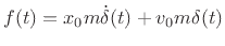
- ... there''.D.3
- Note that, mathematically,
our solution specifies that the mass position is zero prior to time
0. Since we are using the unilateral Laplace transform, there is
really ``no such thing'' as time less than zero, so this is
consistent. Using the
bilateral Laplace transform, the same solution is obtained if
the mass is at position
 for all negative time
, and the
driving force
for all negative time
, and the
driving force  imparts a doublet having ``amplitude''
 at time 0
, i.e.,
at time 0
, i.e.,
 , and all initial conditions are taken to be zero (as they
must be for the bilateral Laplace transform). A
doublet is defined as the time-derivative of the impulse
signal (defined in Eq.(E.5)). In other words, impulsive inputs
at time 0 can be used to set up arbitrary initial
conditions. Specifically, the input
, and all initial conditions are taken to be zero (as they
must be for the bilateral Laplace transform). A
doublet is defined as the time-derivative of the impulse
signal (defined in Eq.(E.5)). In other words, impulsive inputs
at time 0 can be used to set up arbitrary initial
conditions. Specifically, the input
 slams the system into initial state
  at
time 0.
at
time 0.
.
.
.
.
.
.
.
.
.
.
.
.
.
.
.
.
.
.
.
.
.
.
.
.
.
.
.
.
.
.
- ....E.1
- To show this, differentiate the
squared-magnitude frequency response
 with respect to
 , equate to zero, and solve for
. You can see from
checking the denominator of the derivative that the result holds
whenever
, equate to zero, and solve for
. You can see from
checking the denominator of the derivative that the result holds
whenever
 , i.e., as long as there as any amount of decay in
the impulse response (any nonzero bandwidth).
, i.e., as long as there as any amount of decay in
the impulse response (any nonzero bandwidth).
.
.
.
.
.
.
.
.
.
.
.
.
.
.
.
.
.
.
.
.
.
.
.
.
.
.
.
.
.
.
- ...
respectively.E.2
- Exercise: Determine
and
 and
check your result by performing the Laplace transform and comparing to
Eq.(E.7).
and
check your result by performing the Laplace transform and comparing to
Eq.(E.7).
.
.
.
.
.
.
.
.
.
.
.
.
.
.
.
.
.
.
.
.
.
.
.
.
.
.
.
.
.
.
- ...
filters.F.1
- A short tutorial on matrices appears in
[84], available online at
http://ccrma.stanford.edu/~jos/mdft/Matrices.html.
.
.
.
.
.
.
.
.
.
.
.
.
.
.
.
.
.
.
.
.
.
.
.
.
.
.
.
.
.
.
- ...MDFT.F.2
- http://ccrma.stanford.edu/~jos/mdft/Matrix_Formulation_DFT.html.
.
.
.
.
.
.
.
.
.
.
.
.
.
.
.
.
.
.
.
.
.
.
.
.
.
.
.
.
.
.
- ...MDFTF.3
- http://ccrma.stanford.edu/~jos/mdft/
.
.
.
.
.
.
.
.
.
.
.
.
.
.
.
.
.
.
.
.
.
.
.
.
.
.
.
.
.
.
- ... properties.F.4
- http://en.wikipedia.org/wiki/Circulant_matrix
.
.
.
.
.
.
.
.
.
.
.
.
.
.
.
.
.
.
.
.
.
.
.
.
.
.
.
.
.
.
- ... follows:F.5
- While this
example is easily done by hand, the matlab function tf2ss
can be used more generally (``transfer function to state space''
conversion).
.
.
.
.
.
.
.
.
.
.
.
.
.
.
.
.
.
.
.
.
.
.
.
.
.
.
.
.
.
.
- ...
way.F.6
- The methods discussed in this section are intended for
LTI system identification. Many valued guitar-amplifier modes, of
course, provide highly nonlinear distortion. Identification of
nonlinear systems is a relatively advanced topic with lots of special
techniques
[24,17,97,4,86].
.
.
.
.
.
.
.
.
.
.
.
.
.
.
.
.
.
.
.
.
.
.
.
.
.
.
.
.
.
.
- ...
derive.F.7
- There are many possible definitions of pseudoinverse
for a matrix
 . The Moore-Penrose pseudoinverse is perhaps most
natural because it gives the least-squares solution to the set
of simultaneous linear equations
. The Moore-Penrose pseudoinverse is perhaps most
natural because it gives the least-squares solution to the set
of simultaneous linear equations
 , as we show later in
this section.
, as we show later in
this section.
.
.
.
.
.
.
.
.
.
.
.
.
.
.
.
.
.
.
.
.
.
.
.
.
.
.
.
.
.
.
- ...Golub.F.8
- Say help slash in Matlab.
.
.
.
.
.
.
.
.
.
.
.
.
.
.
.
.
.
.
.
.
.
.
.
.
.
.
.
.
.
.
- ... matrix,G.1
- A short tutorial on matrices appears
in [84], available online at
http://ccrma.stanford.edu/~jos/mdft/Matrices.html.
.
.
.
.
.
.
.
.
.
.
.
.
.
.
.
.
.
.
.
.
.
.
.
.
.
.
.
.
.
.
- ...
elsewhere.G.2
- I.e.,
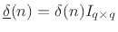 , where
 is the
  identity matrix, and
denotes the
discrete-time impulse signal (which is 1 at time
identity matrix, and
denotes the
discrete-time impulse signal (which is 1 at time  and zero for
all
and zero for
all  ).
).
.
.
.
.
.
.
.
.
.
.
.
.
.
.
.
.
.
.
.
.
.
.
.
.
.
.
.
.
.
.
- ... matrix.G.3
- To emphasize something is a matrix, it is
often typeset in a boldface font. In this appendix, however,
capital letters are more often used to denote matrices.
.
.
.
.
.
.
.
.
.
.
.
.
.
.
.
.
.
.
.
.
.
.
.
.
.
.
.
.
.
.
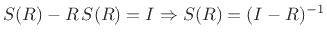
- ... series,G.4
- Let
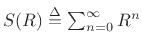 , where
  is a square matrix.
Then
is a square matrix.
Then
 .
.
.
.
.
.
.
.
.
.
.
.
.
.
.
.
.
.
.
.
.
.
.
.
.
.
.
.
.
.
.
.
- ....G.5
- Equivalently, a causal transfer function
 contains a delay-free path whenever
 , since
 .
.
.
.
.
.
.
.
.
.
.
.
.
.
.
.
.
.
.
.
.
.
.
.
.
.
.
.
.
.
.
.
- ...
model.G.6
- An exception arises when the model may be time
varying. A time varying
 matrix, for example, will cause
time-varying zeros in the system. These zeros may momentarily cancel
poles, rendering them unobservable for a short time.
matrix, for example, will cause
time-varying zeros in the system. These zeros may momentarily cancel
poles, rendering them unobservable for a short time.
.
.
.
.
.
.
.
.
.
.
.
.
.
.
.
.
.
.
.
.
.
.
.
.
.
.
.
.
.
.
- ...
quasi-harmonicG.7
- The overtones of a vibrating string are never
exactly harmonic because all strings have some finite
stiffness. This is why we call them ``overtones'' instead of
``harmonics.'' A perfectly flexible ideal string may have exactly
harmonic overtones [55].
.
.
.
.
.
.
.
.
.
.
.
.
.
.
.
.
.
.
.
.
.
.
.
.
.
.
.
.
.
.
- ... form.G.8
- As
of this writing, this function does not exist in Octave or Octave
Forge, but it is easily simulated using sos2tf followed by
tf2ss.
.
.
.
.
.
.
.
.
.
.
.
.
.
.
.
.
.
.
.
.
.
.
.
.
.
.
.
.
.
.
- ...
matlab.G.9
- Specifically, this example was computed using
Octave's tf2ss. Matlab gives a different but equivalent form
in which the state variables are ordered in reverse. The effect is a
permutation given by flipud(fliplr(M)), where
M denotes the matrix A, B, or C. In other
words, the two state-space models are obtained from each other using
the similarity transformation matrix
T=[0 0 1; 0 1 0; 1 0 0] (a simple permutation matrix).
.
.
.
.
.
.
.
.
.
.
.
.
.
.
.
.
.
.
.
.
.
.
.
.
.
.
.
.
.
.
- ... numerically.G.10
- If the Matlab
Control Toolbox is available, there are higher level routines for
manipulating state-space representations; type ``lookfor
state-space'' in Matlab to obtain a summary, or do a search on the
Mathworks website. Octave tends to provide its control-related
routines in the base distribution of Octave.
.
.
.
.
.
.
.
.
.
.
.
.
.
.
.
.
.
.
.
.
.
.
.
.
.
.
.
.
.
.
- ....G.11
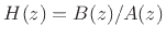
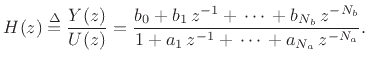
- In general,
we can write an order
Jordan block
 corresponding to eigenvalue
as
corresponding to eigenvalue
as
where  denotes the
  identity matrix, and
Note that  , for
, for
 has ones along the
th
superdiagonal and zeros elsewhere. Also,
has ones along the
th
superdiagonal and zeros elsewhere. Also,
 for
for  .
By the binomial theorem,
.
By the binomial theorem,
where
![$ \left(\begin{array}{c} n \\ [2pt] k \end{array}\right)\isdef n!/[k!(n-k)!]$](img2277.png) denotes the binomial coefficient (also
called ``
choose
'' in probability theory).
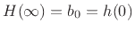
Thus,
denotes the binomial coefficient (also
called ``
choose
'' in probability theory).
Thus,
where the zeros in the upper-right corner are valid for
sufficiently large
, and otherwise the indicated series
is simply truncated.
.
.
.
.
.
.
.
.
.
.
.
.
.
.
.
.
.
.
.
.
.
.
.
.
.
.
.
.
.
.
- ...
matrix.H.1
- Recursive filters are brought into this framework in
the time-invariant case by dealing directly with their impulse
response, or the so called moving average representation.
Linear time-varying recursive filters have a matrix representation,
but it is not easy to find. In general one must symbolically
implement the equation
 and collect coefficients of
  .
.
.
.
.
.
.
.
.
.
.
.
.
.
.
.
.
.
.
.
.
.
.
.
.
.
.
.
.
.
.
.
- ... dc).I.1
- In other
words, matching leading terms in the Taylor series expansion of
 about
about
 determines the poles as a function of the
zeros, leaving the zeros unconstrained. It is shown in
[64] that any filter of the form
determines the poles as a function of the
zeros, leaving the zeros unconstrained. It is shown in
[64] that any filter of the form
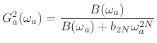
is maximally flat at dc, where
 , with
  necessary
to force a zero at
necessary
to force a zero at
 . Choosing maximum flatness also
at
pushes all the zeros out to infinity, giving the
simple form in Eq.(I.1). It is noted in [64]
how the more general class of Butterworth lowpass filters can be used
to provide maximum flatness at dc while obtaining more general
spectral shapes, such as notches at specific finite frequencies.
. Choosing maximum flatness also
at
pushes all the zeros out to infinity, giving the
simple form in Eq.(I.1). It is noted in [64]
how the more general class of Butterworth lowpass filters can be used
to provide maximum flatness at dc while obtaining more general
spectral shapes, such as notches at specific finite frequencies.
.
.
.
.
.
.
.
.
.
.
.
.
.
.
.
.
.
.
.
.
.
.
.
.
.
.
.
.
.
.
- ... 1947I.2
- See also
the Cayley transform (1846) and Möbius transforms.
.
.
.
.
.
.
.
.
.
.
.
.
.
.
.
.
.
.
.
.
.
.
.
.
.
.
.
.
.
.
- ... Tustin,I.3
- A. Tustin, ``A method of
analysing the behaviour of linear systems in terms of time series,''
J. Inst. Elect. Engrs., Part IIA, Automatic Regulators and Servo
Mech vol. 94, no. 1, May 1947, pp. 130-142
.
.
.
.
.
.
.
.
.
.
.
.
.
.
.
.
.
.
.
.
.
.
.
.
.
.
.
.
.
.
- ... causalI.4
 is said to be causal if
 for
.
for
.
.
.
.
.
.
.
.
.
.
.
.
.
.
.
.
.
.
.
.
.
.
.
.
.
.
.
.
.
.
.
- ... Octave.J.1
- On a Red Hat Fedora
Core Linux system, octave-forge is presently in ``Fedora
Extras'', so that one can simply type yum install
octave-forge at a shell prompt (as root).
.
.
.
.
.
.
.
.
.
.
.
.
.
.
.
.
.
.
.
.
.
.
.
.
.
.
.
.
.
.
- ...
complex):J.2
- Thanks to Matt Wright for contributing the original
version of this example.
.
.
.
.
.
.
.
.
.
.
.
.
.
.
.
.
.
.
.
.
.
.
.
.
.
.
.
.
.
.
- ... language|textbfK.1
- The Faust home page is
http://faust.grame.fr/.
Faust is included in the Planet CCRMA distribution (http://ccrma.stanford.edu/planetccrma/software/).
The examples in this appendix have been tested with Faust version
0.9.9.2a2.
.
.
.
.
.
.
.
.
.
.
.
.
.
.
.
.
.
.
.
.
.
.
.
.
.
.
.
.
.
.
- ... environments.K.2
- Faust
``architecture files'' and plugin-generators are currently available
for Max/MSP, PD [65,31], VST, LADSPA, ALSA-GTK, JACK-GTK,
and SuperCollider, as of this writing.
.
.
.
.
.
.
.
.
.
.
.
.
.
.
.
.
.
.
.
.
.
.
.
.
.
.
.
.
.
.
- ...K.3
- A ``with'' block is not required, but it
minimizes ``global name pollution.'' In other words, a definition and
its associated with block are more analogous to a C
function definition in which local variables may be used.
Faust statements can be in any order,
so multiple definitions of the same symbol are not allowed.
A with block can thus be used also to override global
definitions in a local context.
.
.
.
.
.
.
.
.
.
.
.
.
.
.
.
.
.
.
.
.
.
.
.
.
.
.
.
.
.
.
- ... background.K.4
- Facility with basic C++ programming is also assumed for
this appendix.
.
.
.
.
.
.
.
.
.
.
.
.
.
.
.
.
.
.
.
.
.
.
.
.
.
.
.
.
.
.
- ... signals,K.5
- A
causal signal is any signal that is zero before time 0 (see
§5.3).
.
.
.
.
.
.
.
.
.
.
.
.
.
.
.
.
.
.
.
.
.
.
.
.
.
.
.
.
.
.
- ...cpgr.dsp.K.6
- The faust2firefox script
(distributed with Faust version 0.9.9.3 and later)
can be used to generate SVG block diagrams and open them in the
Firefox web browser.
.
.
.
.
.
.
.
.
.
.
.
.
.
.
.
.
.
.
.
.
.
.
.
.
.
.
.
.
.
.
- ... response:K.7
- This
specific output was obtained by editing cpgrir-print.cpp to replace
%8f by
%g in the print statements, in order to print more
significant digits.
.
.
.
.
.
.
.
.
.
.
.
.
.
.
.
.
.
.
.
.
.
.
.
.
.
.
.
.
.
.
- ...K.8
- In many cases the signal processing in Faust can occur within
a ``foreign function'' written in C or C++ and used as a ``black
box'' within Faust, like the cos() function in
Fig.K.5. However, this approach is presently limited because
foreign functions can have only float and int
argument types, and they can only return a float each sample.
It is possible to set up persistent state in a foreign function by
means of static variables, but this does not generalize easily to multiple
instances.
Therefore, more general extensions may require direct modification of the
generated C++, which usually obsoletes the Faust source code.
.
.
.
.
.
.
.
.
.
.
.
.
.
.
.
.
.
.
.
.
.
.
.
.
.
.
.
.
.
.
- ... patch,K.9
- All manually
generated .dsp files and pd patches in this appendix
are available at
http://ccrma.stanford.edu/realsimple/faust/faustpd.tar.gz.
.
.
.
.
.
.
.
.
.
.
.
.
.
.
.
.
.
.
.
.
.
.
.
.
.
.
.
.
.
.
- ...cpgrui~-help.pd,K.10
- In pd, a dynamically loadable module (pd plugin) is
called an abstraction. (This is distinct from the
one-off subpatch which is
encapsulated code within the parent patch, and which resides in the
same file as the parent patch [66].) It is customary to
document each abstraction with its own ``help patch''. The convention
is to name the help patch ``name-help.pd'', where ``name'' is the name
of the abstraction. Right-clicking on an object in pd and
selecting ``Help'' loads the help patch in a new pd window.
.
.
.
.
.
.
.
.
.
.
.
.
.
.
.
.
.
.
.
.
.
.
.
.
.
.
.
.
.
.
- ...loadbangK.11
- The loadbang object
sends a ``bang'' message when the patch finishes loading.
.
.
.
.
.
.
.
.
.
.
.
.
.
.
.
.
.
.
.
.
.
.
.
.
.
.
.
.
.
.
- ...synth.pd.K.12
- On a Linux system with
Planet CCRMA installed, the command ``locate synth.pd''
should find it, e.g., at
/usr/share/doc/faust-pd-0.9.8.6/examples/synth/synth.pd .
.
.
.
.
.
.
.
.
.
.
.
.
.
.
.
.
.
.
.
.
.
.
.
.
.
.
.
.
.
.
- ... addingK.13
- After running jack-rack, the LADSPA plugin was added
by clicking on the menu items ``Add / Uncategorised / C /
Constant_Peak_Gain_Resonator''. If
jack-rack does not find this or other plugins, make sure your
LADSPA_PATH environment variable is set. A typical setting
would be /usr/local/lib/ladspa/:/usr/lib/ladspa/.
.
.
.
.
.
.
.
.
.
.
.
.
.
.
.
.
.
.
.
.
.
.
.
.
.
.
.
.
.
.
- ...jack-rack-connect.K.14
- Sound routings such as this may be
accomplished using the ``Connect'' window in qjackctl. In
that window, there is an Audio tab and a MIDI tab, and the Audio tab
is selected by default. Just click twice to select the desired
source and destination and then click ``Connect''. Such connections
can be made automatic by clicking ``Patchbay'' in the
qjackctl control panel, specifying your connections,
saving, then clicking ``Activate''. Connections can also be
established at the command line using aconnect from the
alsa-utils package (included with Planet CCRMA).
.
.
.
.
.
.
.
.
.
.
.
.
.
.
.
.
.
.
.
.
.
.
.
.
.
.
.
.
.
.
- ...Receptor|textbf.K.15
- The
Receptor is a hardware VST plugin host designed for studio work and
live musical performance. While it only supports Windows VST
plugins, it is based on a Red Hat Linux operating system using
wine for Windows compatibility. The VST plugin described in
this section was tested on system version 1.6.20070717 running on
Receptor hardware version 1.0. This system expects VST-2.3 plugins,
and so VST-2.4 plugins cause a warning message to be printed in the
Receptor's system log. However, v2.4 plugins seem to work fine in
the 2.3 framework. There was a competitor to the Receptor called
Plugzilla that supported both VST and LADSPA plugins, but Plugzilla
no longer appears to be available.
.
.
.
.
.
.
.
.
.
.
.
.
.
.
.
.
.
.
.
.
.
.
.
.
.
.
.
.
.
.
- ... input.K.16
- Pd must have at least one MIDI-input port
defined at startup for this to work. For example, a typical
~/.pdrc file might contain the following startup options for pd:
-jack -r 48000 -alsamidi -midiindev 1 -midioutdev 1 -audiooutdev 1 -outchannels 2 -path /usr/lib/pd/...
.
.
.
.
.
.
.
.
.
.
.
.
.
.
.
.
.
.
.
.
.
.
.
.
.
.
.
.
.
.
![$\displaystyle \Delta \isdef
\left[\begin{array}{ccccc}
0 & 1 & 0 & \cdots & 0 \\ [2pt]
0 & 0 & 1 & \cdots & 0 \\
\vdots & \vdots & \ddots & \ddots & \vdots \\
0 & 0 & 0 & \ddots & 1 \\ [2pt]
0 & 0 & 0 & \cdots & 0 \\
\end{array}\right].
$](img2271.png)
![\begin{eqnarray*}
J^n \;=\; (pI+\Delta)^n &\!=\!& p^nI + np^{n-1}\Delta
+ \frac{n(n-1)}{2}p^{n-2}\Delta^2
+ \frac{n(n-1)(n-1)}{3!}p^{n-3}\Delta^3 + \cdots \\
& & + \left(\begin{array}{c} n \\ [2pt] k \end{array}\right)p^k\Delta^{n-k}
+ \cdots + np\Delta^{n-1} + \Delta^n,
\end{eqnarray*}](img2276.png)
![$\displaystyle J^n =
\left[\begin{array}{cccccccc}
p^n & np^{n-1} & \frac{n(n-1)}{2} p^{n-2} & \cdots & \cdots & 0 \\ [2pt]
0 & p^n & np^{n-1} & \frac{n(n-1)}{2} p^{n-2} & \cdots & 0 \\
\vdots & & \ddots & \ddots & \ddots & \\
0 & 0 & 0 & & & np^{n-1}\\ [2pt]
0 & 0 & 0 & & & p^n \\ [2pt]
\end{array}\right],
$](img2278.png)