Vector Formulation

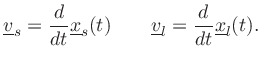
Denote the sound-source velocity by $\underline{v}_s(\underline{x},t)$ where $\underline{x}\isdef (x_1,x_2,x_3)$ is 3D position and $t$ is time. Similarly, let $\underline{v}_l(\underline{x},t)$ denote the velocity of the listener, if any. The position of source and listener are denoted $\underline{x}_s(t)$ and $\underline{x}_l(t)$ , respectively. We have velocity related to position by

$$\underline{v}_s= \frac{d}{dt}\underline{x}_s(t) \qquad \underline{v}_l= \frac{d}{dt}\underline{x}_l(t). \protect$$ (2)

Consider a Fourier component of the source at frequency $\omega_s$ . We wish to know how this frequency is shifted to $\omega_l$ at the listener due to the Doppler effect.

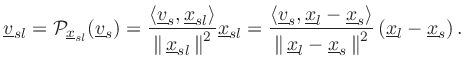
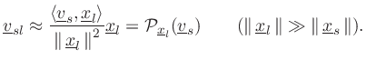
The Doppler effect depends only on the relative motion between the source and listener [12, p. 453]. We must therefore orthogonally project the source and listener velocities onto the vector $\underline{x}_{sl}=\underline{x}_l-\underline{x}_s$ pointing from the source to the listener. (See Fig. for a specific example.)

The orthogonal projection of a vector $\underline{x}$ onto a vector ${\underline{y}}$ is given by [15]

$${\cal P}_{\underline{y}}(\underline{x}) = \frac{\left<\underline{x},{\underline{y}}\right>}{\left\Vert\,{\underline{y}}\,\right\Vert^2}{\underline{y}} \;\isdef \; \frac{\underline{x}^T{\underline{y}}}{{\underline{y}}^T{\underline{y}}}{\underline{y}}$$

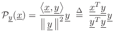
Therefore, we can write the projected source velocity as

$$\underline{v}_{sl}= {\cal P}_{\underline{x}_{sl}}(\underline{v}_s) = \frac{\left<\underline{v}_s,\underline{x}_{sl}\right>}{\left\Vert\,\underline{x}_{sl}\,\right\Vert^2}\underline{x}_{sl} = \frac{\left<\underline{v}_s,\underline{x}_l-\underline{x}_s\right>}{\left\Vert\,\underline{x}_l-\underline{x}_s\,\right\Vert^2}\left(\underline{x}_l-\underline{x}_s\right). \protect$$ (3)

In the far field (listener far away), Eq.$\,$ (3) reduces to

$$\underline{v}_{sl} \approx \frac{\left<\underline{v}_s,\underline{x}_l\right>}{\left\Vert\,\underline{x}_l\,\right\Vert^2} \underline{x}_l = {\cal P}_{\underline{x}_l}(\underline{v}_s) \qquad (\left\Vert\,\underline{x}_l\,\right\Vert\gg\left\Vert\,\underline{x}_s\,\right\Vert). \protect$$ (4)