Rotating Horn Simulation

The heart of the Leslie effect is a rotating horn loudspeaker. The rotating horn from a Model 600 Leslie can be seen mounted on a microphone stand in Fig.4. Two horns are apparent, but one is a dummy, serving mainly to cancel the centrifugal force of the other during rotation. The Model 44W horn is identical to that of the Model 600, and evidently standard across all Leslie models [8]. For a circularly rotating horn, the source position can be approximated as

$$\underline{x}_s(t) = \left[\begin{array}{c} r_s\cos(\omega_m t) \\ [2pt] r_s\sin(\omega_m t) \end{array}\right] \protect$$ (7)

where $r_s$ is the circular radius and $\omega_m$ is angular velocity. This expression ignores any directionality of the horn radiation, and approximates the horn as an omnidirectional radiator located at the same radius for all frequencies. In the Leslie, a diffuser is inserted into the end of the horn in order to make the radiation pattern closer to uniform [8], so the omnidirectional assumption is reasonably accurate.

By Eq.$\,$ (2), the source velocity for the circularly rotating horn is

$$\underline{v}_s(t) = \frac{d}{dt}\underline{x}_s(t) = \left[\begin{array}{c} -r_s\omega_m\sin(\omega_m t) \\ [2pt] r_s\omega_m\cos(\omega_m t) \end{array}\right] \protect$$ (8)

Note that the source velocity vector is always orthogonal to the source position vector, as indicated in Fig..

Figure 3: Relevant geometry for a rotating horn.

Since $\underline{v}_s$ and $\underline{x}_s$ are orthogonal,the projected source velocity Eq.$\,$ (3) simplifies to

$$\underline{v}_{sl}= {\cal P}_{\underline{x}_{sl}}(\underline{v}_s) = \frac{\left<\underline{v}_s,\underline{x}_{sl}\right>}{\left\Vert\,\underline{x}_{sl}\,\right\Vert^2}\underline{x}_{sl} = \frac{\left<\underline{v}_s,\underline{x}_l-\underline{x}_s\right>}{\left\Vert\,\underline{x}_l-\underline{x}_s\,\right\Vert^2}\left(\underline{x}_l-\underline{x}_s\right). \protect$$ (9)

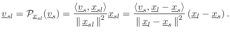
Arbitrarily choosing $\underline{x}_l=(r_l,0)$ (see Fig.), and substituting Eq.$\,$ (7) and Eq.$\,$ (8) into Eq.$\,$ (9) yields

$$\underline{v}_{sl}= \frac{-r_l r_s\omega_m\sin(\omega_m t)}{r_l^2 + 2r_l r_s\cos(\omega_m t)+r_s^2} \left[\begin{array}{c} r_l-r_s\cos(\omega_m t) \\ [2pt] -r_s\sin(\omega_m)t \end{array}\right]. \protect$$ (10)

In the far field, this reduces simply to

$$\underline{v}_{sl}\approx -r_s\omega_m\sin(\omega_m t) \left[\begin{array}{c} 1 \\ [2pt] 0 \end{array}\right]. \protect$$ (11)

Substituting into the Doppler expression Eq.$\,$ (1) with the listener velocity $v_l$ set to zero yields

$$\omega_l = \frac{\omega_s }{1+r_s\omega_m\sin(\omega_m t)/c} \approx \omega_s \left[1-\frac{r_s\omega_m}{c}\sin(\omega_m t)\right], \protect$$ (12)

where the approximation is valid for small Doppler shifts. Thus, in the far field, a rotating horn causes an approximately sinusoidal multiplicative frequency shift, with the amplitude given by horn length $r_s$ times horn angular velocity $\omega_m$ divided by sound speed $c$ . Note that $r_s\omega_m$ is the tangential speed of the assumed point of horn radiation.