The Diagonalized Example System

We can now diagonalize our system using the similarity transformation

$$\mathbf{E}= \left[\begin{array}{cc} \underline{e}_1 & \underline{e}_2 \end{array}\right] = \left[\begin{array}{cc} 1 & 1 \\ [2pt] \eta & -\eta \end{array}\right]$$

where $\eta = \sqrt{\frac{c+1}{c-1}}$ .

We have only been working with the state-transition matrix $\mathbf{A}$ up to now.

The system has no inputs so it must be excited by initial conditions (although we could easily define one or two inputs that sum into the delay elements).

We have two natural choices of output which are the state variables $x_1(n)$ and $x_2(n$ ), corresponding to the choices $\mathbf{C}=[1, 0]$ and $\mathbf{C}=[0, 1]$ :

$$\begin{eqnarray*} y_1(n) &\isdef & x_1(n) \eqsp [1, 0]\, \underline{x}(n)\\ y_2(n) &\isdef & x_2(n) \eqsp [0, 1]\, \underline{x}(n)\\ \end{eqnarray*}$$

Thus, a convenient choice of the system $\mathbf{C}$ matrix is the $2\times 2$ identity matrix.

For the diagonalized system we obtain

$$\begin{eqnarray*} \tilde{\mathbf{A}}&=& \mathbf{E}^{-1}\mathbf{A}\mathbf{E}\eqsp \left[\begin{array}{cc} e^{j\theta} & 0 \\ [2pt] 0 & e^{-j\theta} \end{array}\right] \nonumber \\ \tilde{\mathbf{B}}&=& \mathbf{E}^{-1}\mathbf{B}\eqsp \mathbf{0}\nonumber \\ \tilde{\mathbf{C}}&=& \mathbf{C}\mathbf{E}\eqsp \mathbf{E}\eqsp \left[\begin{array}{cc} 1 & 1 \\ [2pt] \eta & -\eta \end{array}\right] \nonumber \\ \tilde{\mathbf{D}}&=& 0 \end{eqnarray*}$$

where $\theta = \arccos(c)$ and $\eta = \sqrt{\frac{c+1}{c-1}}$ as derived above.

We may now view our state-output signals in terms of the modal representation:

$$\begin{eqnarray*} y_1(n) &=& [1, 0] \underline{x}(n) = [1, 0] \left[\begin{array}{cc} 1 & 1 \\ [2pt] \eta & -\eta \end{array}\right]\tilde{\underline{x}}(n)\\ [10pt] &=& [1, 1]\tilde{\underline{x}}(n) = \lambda_1^n\,\tilde{x}_1(0) + \lambda_2^n\,\tilde{x}_2(0)\\ [20pt] y_2(n) &=& [0, 1] \underline{x}(n) = [0, 1] \left[\begin{array}{cc} 1 & 1 \\ [2pt] \eta & -\eta \end{array}\right]\tilde{\underline{x}}(n)\\ [10pt] &=& [\eta, -\eta]\tilde{\underline{x}}(n) = \eta\lambda_1^n \tilde{x}_1(0) - \eta \lambda_2^n\,\tilde{x}_2(0) \end{eqnarray*}$$

The output signal from the first state variable $x_1(n)$ is

$$\begin{eqnarray*} y_1(n) &=& \lambda_1^n\,\tilde{x}_1(0) + \lambda_2^n\,\tilde{x}_2(0)\\ &=& e^{j\omega_c n T} \tilde{x}_1(0) + e^{-j\omega_c n T}\tilde{x}_2(0) \end{eqnarray*}$$

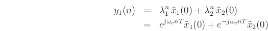
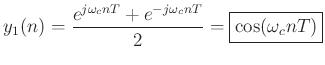
The initial condition $\underline{x}(0) = [1, 0]^T$ corresponds to modal initial state

$$\tilde{\underline{x}}(0) = \mathbf{E}^{-1}\left[\begin{array}{c} 1 \\ [2pt] 0 \end{array}\right] = \frac{-1}{2e}\left[\begin{array}{cc} -e & -1 \\ [2pt] -e & 1 \end{array}\right]\left[\begin{array}{c} 1 \\ [2pt] 0 \end{array}\right] = \left[\begin{array}{c} 1/2 \\ [2pt] 1/2 \end{array}\right]$$

For this initialization, the output $y_1$ from the first state variable $x_1$ is simply

$$y_1(n) = \frac{e^{j\omega_c n T} + e^{-j\omega_c n T}}{2} = \zbox{\cos(\omega_c n T)}$$

Similarly $y_2(n)$ is proportional to $\sin(\omega_c n T)$
(``phase quadrature'' output), with amplitude $\eta$ .