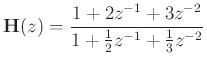
Next  |  Prev  |  Up  |  Top  |  JOS Index  |  JOS Pubs  |  JOS Home  |  Search

Converting to State-Space Form by Hand

  1. First, determine the filter transfer function $ \mathbf{H}(z)$ . In the example, the transfer function can be written, by inspection, as

    $\displaystyle \mathbf{H}(z) = \frac{1 + 2 z^{-1}+ 3 z^{-2}}{1 + \frac{1}{2}z^{-1}+ \frac{1}{3}z^{-2}}
$

  2. If $ {\mathbf{h}}(0)\neq 0$ , we must ``pull out'' the parallel delay-free path:

    $\displaystyle \mathbf{H}(z) = d_0 + \frac{b_1 z^{-1}+ b_2 z^{-2}}{1 + \frac{1}{2}z^{-1}+ \frac{1}{3}z^{-2}}
$

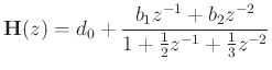
    Obtaining a common denominator and equating numerator coefficients yields

    \begin{eqnarray*}
d_0 &=& 1\\
b_1 &=& 2 - \frac{1}{2}= \frac{3}{2}\\ [10pt]
b_2 &=& 3 - \frac{1}{3}= \frac{8}{3}
\end{eqnarray*}

    The same result is obtained using long or synthetic division

  3. Next, draw the strictly causal part in direct form II, as shown below:

    \begin{center}
\epsfig{file=eps/ssexdf.eps,width=\textwidth } \\
\end{center}

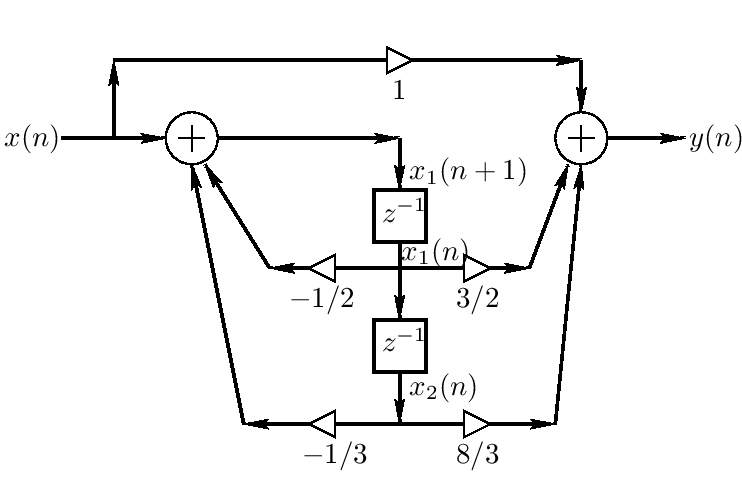
    It is important that the filter representation be canonical with respect to delay, i.e., the number of delay elements equals the order of the filter

  4. Assign a state variable to the output of each delay element (see figure)

  5. Write down the state-space representation by inspection. (Try it and compare to answer above.)


Next  |  Prev  |  Up  |  Top  |  JOS Index  |  JOS Pubs  |  JOS Home  |  Search

Download StateSpace.pdf
Download StateSpace_2up.pdf
Download StateSpace_4up.pdf

``Introduction to State Space Models'', by Julius O. Smith III, (From Lecture Overheads, Music 420).
Copyright © 2019-02-05 by Julius O. Smith III
Center for Computer Research in Music and Acoustics (CCRMA),   Stanford University
CCRMA  [Automatic-links disclaimer]