import numpy as np
import matplotlib.pyplot as plt
from matplotlib.lines import Line2D
import audio_dspy as adsp

import SchemDraw
from SchemDraw import dsp
import SchemDraw.elements as e

import random as r
from scipy.stats import norm
Bad Circuit Modelling
I want to start by addressing something I've heard a few times in the world of virtual analog modelling for digital audio effects. Let's say I wanted to make a model of the famous LA-2A optical compressor. So I buy an actual LA-2A, I take measurements, analyze the circuit diagrams, etc, and construct a virtual model of the effect. In recent years, modelling accuracy has reached the point where it is possible to construct a model that sounds more like my unit than my unit sounds compared to another unit of the same make.
In the analog modelling world, this level of precision is often considered a great success, and without a doubt, achieving that level of precision is certainly a great feat of engineering, requiring a deep knowledge of the system being modelled, as well as incredible attention to detail. However, from an audio perspective, I would consider this result somewhat of a failure.
When I buy an LA-2A, I an buying a unique piece of hardware, that sounds unlike anything else in the world. This uniqueness, particularly when compounded across the many effects used in a production, can give my sounds an interesting character that is specific to my studio. On the other hand if I use a software model of an LA-2A, the version on my computer will sound exactly the same as everyone else's. For some mixing engineers this uniformity is seen as a good thing: if I go to someone else's studio and they have the same plugins as I do, I can be assured they will sound exactly the same as I am accustomed to. That said, in my experience as a mixing engineer, the variations in hardware effects can add a ton of positive elements to a mix, including stereo width, perceptual depth, and once again, a characteristic sound of my studio.
In this series, I'm planning to explore some of the elements that can cause variations in analog effects. While I plan to focus mostly on basic electrical components (resistors, capacitors, etc), similar ideas can usually be applied to more complex circuit elements, as well as other analog audio elements including speaker cones, guitar strings, magnetic tape, and more.
Component Tolerances:

In this article, we'll be talking about component tolerances, one of the most fundamental causes of variations in analog circuits. The basic idea is that no electrical component can be manufactured with perfect precision. With that in mind, manufacturers label their parts with a tolerance rating. So if you buy a 500 Ohm resistor, the resistor will also have a tolerance rating, say +/- 5%, or +/- 1%, or something of the sort. In general, for a more precise overall circuit, it is better to use parts with lower tolerance ratings, however, such parts are also more expensive, so circuit designers try to build robust designs that can handle a little bit of component variation, and will often optimize their circuit to find a balance between cost and precision.
Circuit Analysis
As an example of this phenomenon, let's analyze and construct a model of an ideal Sallen-Key second-order lowpass filter.
L = 2
d = SchemDraw.Drawing(fontsize=12, color='white')
op = d.add(e.OPAMP, flip=True)
d.add(e.LINE, d='left', l=1.75, xy=op.in2)
R2 = d.add(e.RES, d='left',l=L, label='R')
R1 = d.add(e.RES, d='left',l=L, label='R')
d.add(e.DOT, label='Input')

d.add(e.DOT_OPEN, xy=R2.start)
d.add(e.CAP, d='down', l=L, label='C')
d.add(e.GND)

d.add(e.DOT_OPEN, xy=R2.end)
d.add(e.LINE, d='up', l=1.5)
d.add(e.CAP, d='right', tox=op.out+1, label='C')
d.add(e.LINE, d='down', toy=op.out)
d.add(e.DOT_OPEN)

d.add(e.LINE, d='left', l=0.5, xy=op.in1)
d.add(e.LINE, d='down', l=1.25)
vm = d.add(e.DOT_OPEN)
d.add(e.RES, d='down', l=L, label='R1')
d.add(e.GND)
d.add(e.RES, xy=vm.start, d='right', label='R2', tox=op.out+0.5)
d.add(e.LINE, d='up', toy=op.out)
d.add(e.DOT_OPEN)

d.add(e.LINE, d='right', xy=op.out, l=2)
d.add(e.DOT, label='Output')

d.draw()
Note that in this idealized model, we will assume that the op-amp provides perfect, linear gain, as opposed to the more nonlinear response that might be observed in real life. From this model, we can can calculate the cutoff frequency and Q value for the filter as follows:
$$ f_c = \frac{1}{2 \pi R C} $$ $$ Q = \frac{1}{2 - \frac{R_2}{R_1}} $$
Now let's design our example filter such that $f_c = 1 \text{ kHz}$, and $Q = 2$. In other words, we choose $C = 4.7 \text{ nF}$, $R = 33.8 \text{ kOhms}$, $R_2 = 1.5 \text{ kOhms}$, and $R_1 = 1 \text{ kOhms}$. When we construct a digital model of this filter we obtain the following frequency response.
def getCompVal(val, tol):
    if tol == 0:
        return val
    stddev = val * tol / 2
    return r.gauss(val, stddev)

def design_SKLPF(R, C, R1, R2, fs, tol=0):
    fc = 1.0 / (2 * np.pi * getCompVal(R, tol) * getCompVal(C, tol))
    Q = 1.0 / (2 - (getCompVal(R2, tol) / getCompVal(R1, tol)))

    return adsp.design_LPF2(fc, Q, fs)

fs = 44100
b, a = design_SKLPF(4.7e-9, 33800, 1000, 1500, fs)
adsp.plot_magnitude_response(b, a, fs=fs)
plt.ylim(-60)
plt.title('Sallen-Key LPF')
Inserting Imperfections
Now let's see what happens when we make our circuit elements less perfect, specifically by including component tolerances as part of our model. For now we'll use a Gaussian distribution for the randomness of our component values, but we'll discuss more realistic distributions in more detail later on.
The following plot demonstrates how the frequency response varies for different levels of component tolerance:
for n in range(1000):
    b, a = design_SKLPF(4.7e-9, 33800, 1000, 1500, fs, tol=0.1)
    l, = adsp.plot_magnitude_response(b, a, fs=fs)
    l.set_color((1.0, 0.0, 0.0, 0.5))

b, a = design_SKLPF(4.7e-9, 33800, 1000, 1500, fs)
la, = adsp.plot_magnitude_response(b, a, fs=fs)
la.set_color('cyan')
la.set_linewidth(2.5)

custom_lines = [Line2D([0], [0], color='cyan', lw=1),
                Line2D([0], [0], color=(1.0, 0.0, 0.0, 1.0), lw=1)]

plt.title ('Sallen Key LPF with 10% tolerance (Gaussian)')
plt.legend(custom_lines, ['Ideal', r'$\pm$10%'])

plt.ylim(-60)
Now I should note that the above plot is a little bit of an exaggeration, with regards to the actual variations present in analog hardware. First off, 10% is a pretty large tolerance, and one would expect manufacturers, particularly those who make high-end gear, to use higher quality parts. Additionally, most respectable hardware makers have some form of quality control both in rejecting abnormally bad components before including them in their circuits, as well as testing their completed products before they are shipped. So the actual variation in a lowpass filter circuit that you might buy should never be quite as bad as that shown in the plot above, but the basic idea that such variation exists definitely still stands.
Probability Distributions
When I first started looking at this idea of introducing component tolerances into circuit models, I had expected the actual component values to follow a more or less Gaussian distribution. The reality turns out to be a bit more complicated. Although there appears to be a lack of academic writing on the subject, engineers and hackers seem to agree that actual component values follow something like a "truncated Gaussian" distribution. The interested reader is encouraged to read this insightful and humorous article on the subject from Howard Johnson [link].
def trunc_gauss(x, mu, sig, start, end):
    y = np.zeros(len(x))
    ind = np.argwhere(np.logical_and(np.abs(x-mu) < end, np.abs(x-mu) > start))
    y[ind] = norm.pdf(x[ind], mu, sig)
    return y

R = 1000
diff = 200
tol_low = 0.05
tol_high = 0.1
x = np.arange(R-diff, R+diff, 0.1)
y = adsp.normalize(trunc_gauss(x, R, 50, R*tol_low, R*tol_high))
plt.plot(x, y)

plt.xlabel('Resistance [Ohms]')
plt.ylabel('Probability')
plt.title('Probability Distribution of 1 kOhm Resistor with 10% tolerance')
Now we can see what our new frequency responses should look like with our updated component value distribution.
def getCompVal2(val, tol_low, tol_high):
    if tol_high == 0:
        return val
    stddev = val/10

    return_val = 0
    while np.abs(return_val-val) > val*tol_high or np.abs(return_val-val) < val*tol_low:
        return_val = r.gauss(val, stddev)
    return return_val


def design_SKLPF2(R, C, R1, R2, fs, tol=0):
    fc = 1.0 / (2 * np.pi * getCompVal2(R, tol/2, tol) * getCompVal2(C, tol/2, tol))
    Q = 1.0 / (2 - (getCompVal2(R2, tol/2, tol) / getCompVal2(R1, tol/2, tol)))

    return adsp.design_LPF2(fc, Q, fs)

for n in range(1000):
    b, a = design_SKLPF2(4.7e-9, 33800, 1000, 1500, fs, tol=0.1)
    l, = adsp.plot_magnitude_response(b, a, fs=fs)
    l.set_color((1.0, 0.0, 0.0, 0.5))

b, a = design_SKLPF2(4.7e-9, 33800, 1000, 1500, fs)
la, = adsp.plot_magnitude_response(b, a, fs=fs)
la.set_color('cyan')
la.set_linewidth(2.5)

custom_lines = [Line2D([0], [0], color='cyan', lw=1),
                Line2D([0], [0], color=(1.0, 0.0, 0.0, 1.0), lw=1)]

plt.title ('Sallen Key LPF with 10% tolerance (Trunc. Gaussian)')
plt.legend(custom_lines, ['Ideal', r'$\pm$10%'])

plt.ylim(-60)
Implementation
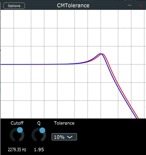
Now for an audio plugin to include component tolerances, is actually a pretty simple matter. As an example, I've developed a simple plugin that models the Sallen-Key lowpass filter circuit from above, and includes an option to change the component tolerances. In my implementation, the values of each component for each tolerance are calculated when the plugin is initialized, using the truncated Gaussian distribution. Another option could be for plugin manufacturers to generate some sort of random seed from the registration or installation process of their plugin, so your copy of their plugin will sound the same every time you use it, but will sound different from everybody elses.
Another important thing to consider (in my opinion), is to use different components for the two channels of a stereo effect, so that for tolerance values greater than zero, the circuits being modelled between the two channels is not exactly the same. For large component tolerances, this stereo mismatch can make the effect seem unbalananced, and sort of "lean" to one side, however for smaller values it still sounds correct, while lending the sound a little bit of extra stereo "width", that would be missing otherwise.
Finally...
That's all for today's article, thanks for reading! For my next article, I'm planning to examine the effects of aging on electrical components, and see how that affects our models of audio effect circuits.