In recent years, there has been a great deal of work on using non-negative spectrogram factorization techniques to model audio. Although these methods can work quite well in certain situations, they have several limitations. One of the main limitations is that they ignore the non-stationarity of audio and temporal dynamics. We have developed new models that address this.

Non-negative spectrogram factorization refers to a class of methods including non-negative matrix factorization and probabilistic latent component analysis (PLCA), that are used to factorize spectrograms. In this discussion, we will use the specific case of PLCA. However, the ideas generalize to most such methods.

These methods are particularly useful to model sound mixtures. The basic idea is that each source is modeled as a linear combination of spectral components (vectors) from a single dictionary. The mixture is in turn modeled as a linear combination of the individual sources. Therefore, the mixture is effectively modeled as linear combination of spectral components from a concatenation of the individual dictionaries.

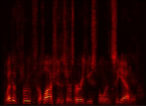
Let us first examine the effectiveness of modeling a single source with a single dictionary, using PLCA. We start with the following simple example of a clip of five piano notes.

Of the five notes, this clip has four distinct notes. It is therefore reasonable that it is explained by a dictionary of four spectral components, which is represented below.

One of the problems with this representation is that it represents each note by a single spectral component. This does not account for the variations in each individual note (attack, decay, etc.). One way to circumvent this issue is to use a much larger dictionary, as shown below.

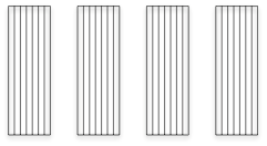
Although, this will do a better job of modeling the variations in an individual note, there are a few issues with the solution. Audio is non-stationary and this modeling strategy does not account for that. Even though we need a larger number of spectral components to model each note, only one of the notes is primarily active at a given time. It would therefore be desirable to have a separate set of statistics (dictionary) to model each note as shown below. We would still have multiple spectral components to model the variations in each note.

Dictionary of four spectral components

Large dictionary

This has multiple advantages over using a single large dictionary. When we have multiple small dictionaries, each time frame will be explained mainly by a single dictionary. Therefore, when it comes to modeling mixtures of sounds, even if two sounds have similar global spectral characteristics, we can still achieve a fairly good separation as long as they don’t have the same spectral characteristics at the same time. For example, in speech separation of two speakers, even though the overall spectral characteristics of the two speakers might be the same, it is quite likely that two speakers will not be speaking the same phoneme at the same time.

Another advantage of having multiple small dictionaries is that in certain applications, we can process or analyze each individual note.

The next advantage is that there is a structure to the non-stationarity in audio. This is explained by temporal dynamics. We therefore explicitly model the temporal dynamics using a Markov Chain. Each state of the Markov chain corresponds to a dictionary. This brings us to the proposed model, the non-negative hidden Markov model (N-HMM), that is shown below. Given a spectrogram, all of the dictionaries as well as the Markov chain can be jointly learned using parameter estimation in the N-HMM.

Four small dictionaries

Non-negative Hidden Markov Model

Without getting into the specific details, the graphical model for PLCA and the N-HMM are shown below. The important thing over here is that in the N-HMM, we see arrows between time frames. This corresponds to modeling temporal dynamics. In contrast, each time frame is independent, in PLCA. This is the case with non-negative spectrogram factorization techniques in general.

Non-negative Hidden Markov Model

PLCA

Now let’s consider another simple example. The following clip is a synthesized saxophone playing four repetitions of an ascending C major arpeggio (the constant Q transform has been used for clarity of display purposes but the algorithm was run on the spectrogram).

We model the above clip using the N-HMM. We estimate the dictionaries and a transition matrix to explain the data. It should be noted that we do not perform any segmentation of the data or use isolated notes for the learning. We merely tell the algorithm to use 3 dictionaries to explain the data. It figures out the segmentation automatically. In order to illustrate this, we perform a reconstruction of the contributions from each of the 3 dictionaries, as shown below.

As we can see and hear, the parameter estimation has correctly used one dictionary to explain each note. The transition matrix is shown below. It tells us that if we are in a given note, there is a high probability of staying in the same note, a small probability of moving to one other note, and a zero probability of moving to the other of the two notes.

t

t + 1

0

0.0698

0.9048

0.093

0.9302

0

0.907

0

0.0952

Once we perform the reconstruction above, we can process or analyze the notes individually. We use this for content-aware audio processing. We flatten the third by a semi-tone and put the notes back together. This is effectively changing the C major arpeggio into a C minor arpeggio as shown below.

We now move onto another more complicated example. The input data (shown below) is nine sentences of speech from a single speaker (from the TIMIT database).

C major arpeggios

Reconstructions from dictionaries

Transition Matrix

C minor arpeggios

Nine sentences of speech

We model this data using the N-HMM. We tell the the algorithm to learn 40 dictionaries of 10 spectral components each, as shown below. The only input to the algorithm are these two parameters.

We see that each each dictionary roughly corresponds to a subunit of speech, as expected.

The estimated transition matrix is shown below. The strong diagonal shows that the model learns state persistence as expected.

Learned dictionaries

Transition Matrix

We now move onto sound mixtures. Lets start with a simple example in which each source is explained by two dictionaries. When we model the mixture, a given time frame of a given source can be explained by one of its two constituent dictionaries. The mixture can therefore be modeled by any one of four combinations of dictionaries as shown below.

Dictionary of sound mixtures

We propose a new model, the non-negative factorial hidden Markov model (N-FHMM) to model mixtures as described above. The graphical model for two sources is shown below. The graphical model of two individual N-HMMs (one on the top and one on the bottom) can be seen.

Non-negative Factorial Hidden Markov Model

We apply these models to supervised source separation. The procedure is as follows:

1. • Learn an N-HMM model (dictionaries and transition matrix) of each source using training data of that source.
   

2. • Model the mixture (which contains unseen test data) using the N-FHMM. The dictionaries and transition matrix of each source will be pre-specified.
   

3. • Learn a set of weights for the mixture components.
   

4. • Reconstruct the two sources.
   

We applied this method to speech separation. The dictionaries and transition matrix that was learned for each source is much like the speech example shown above.

An example of the speech data that we separate is below.

Once we perform source separation, we get the following separated sources.

Speech Mixture

Separated male speaker

Separated female speaker

As a comparison, we performed the same supervised source separation experiment using non-negative spectrogram factorization (PLCA). We then repeated the same experiment with seven other pairs of speakers. We evaluated the quality of the separation using the metrics defined in the BSS-EVAL toolbox. We report the average metrics over all eight pairs of speakers in the table below. We report the metrics in the case in which we use 10 components per dictionary (K=10) as well as the case in which we use 1 component per dictionary (K=1), in the proposed model.

SAR

(dB)

SDR

(dB)

Proposed model (K=10)

Proposed model (K=1)

8.65

7.95

4.82

12.07

7.26

5.58

PLCA

14.07

7.74

6.49

SIR

(dB)

We see a large improvement in the actual suppression of the unwanted source (SIR). We however see a small increase in the introduced artifacts (SAR). The results intuitively make sense. The N-FHMM performs better in suppressing the competing source by enforcing a reasonable temporal arrangement of each speaker’s dictionary elements, therefore not simultaneously using dictionary elements that can describe both speakers. On the other hand, this exclusive usage of smaller dictionaries doesn’t allow us to model the source as well as we would otherwise (with 1 component per dictionary being the extreme case). There is therefore an inherent trade-off in

the suppression of the unwanted source and the reduction of artifacts.

The sound files of the separation results for all eight pairs of speakers can be found here .

References

1. • G. J. Mysore, “A Non-negative Framework for Joint Modeling of Spectral Structure and Temporal Dynamics in Sound Mixtures” . Ph.D. Thesis, Stanford University. June 2010
   

1. • G. J. Mysore, P. Smaragdis, B. Raj, “Non-negative Hidden Markov Modeling of Audio with Application to Source Separation”, In Proceedings of the International Conference on Latent Variable Analysis and Signal Separation (LVA / ICA), St. Malo, France. September 2010
   

     Best Student Paper Award