Inducing Unusual Dynamics in Acoustic Musical Instruments
Sound Examples and Additional Info
Edgar Berdahl
September, 2007
This is the website corresponding to the paper:
Brief note on resonant ring modulation:
Websites for related conference papers:
I. Examples With Multiple Equilibria

Figure 1. Ten plucks with linearly increasing magnitude (above), Corresponding
loop gain L(t) (below)
Fig. 1 shows the results from the simulation where the string is
virtually plucked ten times with initial conditions corresponding to increasing
magnitudes. Fig. 1 (top) demonstrates that the final
equilibrium RMS state depends on the initial condition. Four different stable
equilibria in xp are evident.
Fig. 1 (bottom) reveals that for each pluck, the loop gain L
first wraps around a number of times while the energy outside the main resonances decays,
and then L converges to the value inducing marginal stability as desired.
Because velocity feedback is used instead of the integral of displacement
feedback, the balance between the energy in the various harmonics does not change much even as the level is driven to a target.
| The RMS level is quickly driven to a neighboring target.
Some slight distortion may be heard directly following the attacks. This
corresponds to L(t) varying wildly as the level detector first starts
seeing the transient.
|
II. Band-Pass Filter Effect
The bandpass filter effect may also be used advantageously to control the RMS level
of a single
mode without affecting others. This involves tuning a high-Q band-pass
filter (two-pole, no zeros) to the mode in question.
| Here the
band-pass filter is tuned to the second harmonic. Positive
feedback is applied in order to damp the second harmonic quickly. The other
harmonics remain unchanged.
|
| This is the same as above, except that negative
feedback is applied to increase the decay time constant of the second harmonic.
|
The block diagram in Fig. 2 shows in particular how multiple channels may be
connected together to control multiple harmonics simultaneously.

Figure 2. System block diagram for implementing
multiple level-regulating
controllers concurrently
The 1st, 2nd, 3rd, 4th, 5th, 6th, 9th, and 10th harmonics were controlled
simultaneously in order to make the vibrating string model sing. To this end,
they were driven to the spectral envelope outlined by the three formants f1,
f2, and f3 for the the short u and a vowels. Since the sensor
and actuator were placed realistically in the model accoring to real physical
characterstics, both the 7th and 8th harmonics are both harder to sense and
actuate. This is a controllability/observability problem due to the sensor and
actuator being placed near a node for the 7th and 8th harmonics. Thus, we did not attempt to control them due to signal to noise
ratio considerations (see discussion regarding Fig. 5). This means that the formants are not
perfectly modeled, but it still should be possible to hear which vowel is being
"sung." Fig. 3 shows the performance of the controller for the second
harmonic. The initial pluck at t=0s causes some overshoot of the target
and the loop gain L2 to be underestimated. However, soon the disturbance
subsides and the controller adapts to the correct loop gain using the
adaptive controller. Then at t=5s, the target vowel switches from
u to a. After a few seconds, the RMS level is again driven to
the correct target. Of course in both cases the same loop gain is used to
induce marginal stability as soon as the target RMS level is achieved.

Figure 3. Driving the RMS of the second harmonic to 135 until
t=5, at which
point the RMS is driven to 24
The match of the spectra was quite good. Fig. 4 shows the spectrum in blue of
x at the end of the u vowel after the system has nearly converged to the
steady-state solution. The red circles are the targets as specified by the
formants of the vowel.
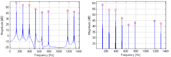
Figure 4. Match between the desired levels and the attained levels (left,
zoomed out; right, zoomed in)
The match is quite good (within +/-1.5dB) given the controller is non-ideal in some ways. For
example, band-pass filters that are not perfectly tuned to the harmonic will
impart a gain error. This means that, even though the adaptive controller
for a given harmonic believes it has achieved the target, it may be slightly
off-target because the band-pass filter is mistuned. Another non-ideality is
that dividing signals by RMS level estimates leads to some harmonic
distortion. Fig. 5 shows the spectrum of the nearly steady-state signal
u1, which is the control signal for the first harmonic, as
estimated from the same time frame as Fig. 4.

Figure 5. Spectrum of steady-state signal
u1
| This is the
sound of the eight harmonics being controlled as explained above to synthesize a u and then
an a vowel.
|
| This is essentially the same example except
that some modulation has been added because this aids in perceiving vowels. In
particular, the error signals were slightly amplitude modulated at 1Hz.
|
III. Resonant Ring Modulation

Figure 6. RMS levels for resonant ring modulation
Resonant ring modulation involves amplitude modulating the feedback signal by a
sinusoid with carrier frequency fc. For more information,
see an Analysis Of Resonant Ring Modulation. One
difference here, which holds for all of the following examples except for the
last two, is that an additional first-order low-pass filter is applied in
the feedback loop preceeding the modulation to form the effect. This helps
improve the sound quality by preventing too much energy from being stored in
the higher harmonics.
Here fc is swept linearly from f0 to 2.05f0:
| In this case, the loop gain L is held constant. This
corresponds to the blue line in Fig. 6. Note how the quieter sections sound
somewhat hollow because the controller is not driving the plant hard enough
during these sections. This example has a noticeable pluck at the beginning
because the loop gain L begins at the constant.
|
| This time, the adaptive controller is applied to drive
the RMS level to a target. This not only reduces the dynamic range of the
instrument's output, but it also helps shift the applied parameters closer to
the space of interesting-sounding ones. For instance, this sound does not
contain any "hollow"-sounding sections. Note that this example does not have a
noticeable pluck at the beginning because the loop gain L begins at zero.
|
Here fc is swept linearly from f0 to 4.05f0:
| Now fc
is swept over a much larger range revealing more parts of the space with unique
dynamics. The adaptive controller is applied here.
|
| This is the same as above, except that we are listening
to a limited version of the feedback signal rather than the output from the
string itself. Note that as a result, it sounds less resonant because we do
not tend to hear the natural string harmonics ringing out because they are
instead modulated.
|
For the last two examples, the simplest form of resonant ring modulation is
implemented. That is, there is no low-pass filter in the feedback loop, and so
the sound examples may sound tinny due to the additional higher-frequency content:
| Here we
have another example of a three octave sweep using the adaptive controller.
|
| This is the example
from the note on resonant ring modulation. We can hear the
partials converge to the target spectrum.
|
