Since
everything is a filter, people talk frequently about impulse responses but rarely actually measure them. In fact, at the beginning of the class, we measured the impulse response of the slap-back echoes between two of the CCRMA trailers, but I was interested in measuring the impulse responses of EQ-filters, which are generally simpler. I originally wanted to use maximum length sequences (MLS) to make the measurement because they provide accurate results, but complications arose because these sequences are
2M - 1 samples long where
M is an integer, while FFTs are much more compatible with lengths such as
2M. Maximum length sequences can not be zero (or otherwise) padded to attain a length of
2M without destroying the flatness of their amplitude spectra. See the papers on impulse response measurement at the bottom of
this page.
I decided to investigate the use of adaptive filters to measure impulse responses. While experimenting with MATLAB, I found that the algorithm was quite robust, so I implemented an external for
Miller Puckette's
Pd. To make the code more-easily portable for
Cycling '74's
Max/MSP, I wrote the code using
flext, which abstracts the external-writing process. In retrospect, I would recommend flext for those writing simple externals; however, more complicated externals require understanding the underlying C interpretation. This is because flext causes C code to be generated, and any error messages that the compiler generates will be related to the underlying C code.
The adaptive filter takes the input signal
x(n), which is ideally a kind of white noise, in the leftmost inlet. In fact, white noise consisting of only 1's and -1's is best because it will increase the SNR of the measurement. However, the algorithm that the adaptive filter uses works so well that signals besides white noise will often produce reasonable results as long as they contain energy in most parts of the spectrum. The algorithm begins by convolving
x(n) with the approximate impulse response
h(j) that it is measuring. Note that
h(j) is assumed to be of length
N and can be interpreted as an FIR filter. If impulse response being measured is actually longer than
N, then the algorithm will find the best approximating FIR filter of length
N.
b(n), which should be connected to the rightmost inlet, is the signal resulting from passing x(n) through the system being measured. The algorithm finds the error e(n) by subtracting b(n) from z(n).
Let Q(n) be the square of the error.
And minimize the square of the error by setting its derivative with respect to each of the filter coeffiecients to zero. The solution turns out to be quite simple.
The solution can be approximated iteratively. When the algorithm is started,
h(j,0) = 0 for all
j, and then the filter coefficients are allowed to vary as described below.

controls the speed of the adaption per iteration. A reasonable value for
is 0.05.

The first
Pd example patch shows a simple demonstration of the filter. The user can draw an FIR filter of length 64 in the array shown in the upper righthand corner. Then, after the user clicks the "animate" toggle, the adaptive filter's approximation will be shown in the lower lefthand corner. This is because everytime the user sends the adaptive filter the "show" message, it updates the contents of the array assigned to it (including the length of the array if it has been changed). If the user chooses a small
, then the filter will adapt so slowly that the user can actually watch it adapt. In fact, if the user selects the appropriate toggle switches, then the user can listen to
z(n) as the filter adapts over time. If
is chosen somewhat larger, then the filter will adapt very quickly. However, it is also possible for the user to pick
so large that the filter no longer converges. To prevent especially unpleasant results such as loud popping sounds and NaN's that propagate through the DSP chain, I added a few lines of code that occassionally check the filter coeffients
h(j) to make sure that they remain in the range [-5 5].

By switching the two inputs (
x(n) and
b(n)) and delaying the unfiltered input by 32 samples, this
Pd patch can actually be used to find the optimal inverse FIR filter, which must be stable since it is FIR. The image below shows an example where the FIR filter to be inverted consists of only two positive taps, and is thus a very simple FIR filter. The actual inverse filter must be IIR by nature, but it can be approximated by an FIR filter as shown below. Note that since the filter coefficients for the adaptive filter are stored in an array, they can be easily saved to disk.
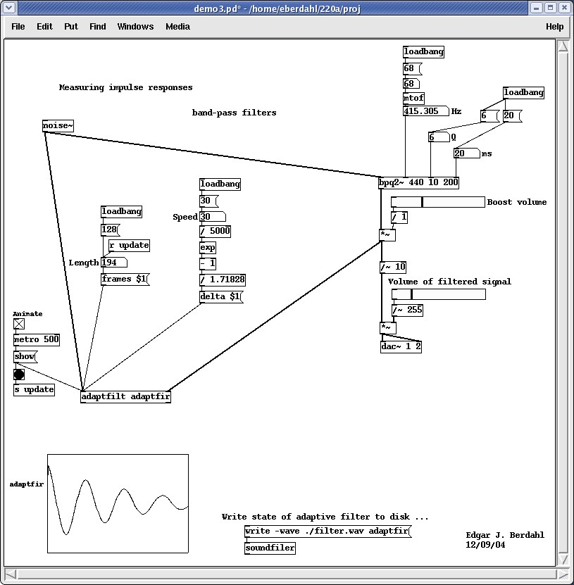
This
example Pd patch shows what the impulse response of a bandpass filter looks like: a damped exponential. Increasing the Q of the filter decreases both the amplitude and the damping coefficient of the impulse response.
The final
example Pd patch shows what happens when the adaptive filter is abused. The object expects to receive two inputs that are closely related and attempts to find a short FIR filter that it can convolve with one input to approximate the other. If the two input signals are two unrelated, or the delay between them is longer than
N, then the adaptive filter will not converge; however, the output
z(n) may sound quite interesting. In fact, if
is increased such that the filter adapts quickly,
z(n) sounds roughly like the convolution of
x(n) and
b(n) but with some randomness introduced by the filter coefficients not being able to find optimal values. This time-domain convolution effect is advantageous for low-latency situations, where the FFTs typically used for convolving two changing signals introduce extra latency.

Hints:
The convolution inherent in the adaptive filter algorithm causes a fairly heavy CPU load. For example, on my 2.8GHz Pentium IV, I can increase
N to about 300 taps before audio dropouts occur.
- Run as few other programs in the background as possible.
- Set the sampling rate to 22kHz.
- Turn the "animate" toggle switch off. To see the current adaptive filter coefficients, click on the "show" message.
- Make the audio vector size as large as possible.
- If audio dropouts are not a problem, N can usually be increased much more for the purpose of making measurements. This is because the algorithm is so robust that even when it is interrupted some of the time, the filter coefficients h(j) still converge.
Future ideas:
- Increase the efficiency of the algorithm by using bit-shifting operations instead of multiplies. The trick is that the filter coefficients h(j) still converge even when only the signs of e(n) and x(n-j) are used.
- Implement a mode where the adaptive filter can assume that x(n) consists only of 1's and -1's. In this case, the multiplies in the convolution for producing z(n) could be converted to additions and subtractions. In this mode, the adaptive filter would be less general, but it would be much more efficient, especially in combination with the optimization described above. Then memory accesses would probably become the largest factor limiting the size of N.
- Use Golay codes to measure the impulse responses. Because they are of length 2M, FFTs can be more easily applied to find the approximate impulse response of the system. They would not be able to change as quickly as the adaptive filters, but they would also work for much larger values of N.


