WEEK 1 - BACKGROUND

In reaction to the violence of Vietnam War protests and JFK assassination in 1973, Pauline Oliveros embarked on the Meditation Project, a 10-week-long experiment with 20 participants. Each day, they practiced body awareness, tai chi, karate, calligraphy, yoga, and Oliveros' Sonic Meditations, with the goal of healing human consciousness, fostering connections, and increasing relatedness. Before and after the experiment, Oliveros collected qualitative and quantitative data to measure changes. The Betts Test was used to measure sensory modalities including visual, auditory, kinesthetic, and tactile. The Seashore Test was used to measure musical skills including pitch, loudness, rhythm, timbre, time, and tonal memory. Although she hypothesized that sensory awareness and musical skills would increase, Tysen Dauer's statistical analyses revealed no significant differences. He remarks that this may be due to the fact that participants were not trained on the skills measured by the Seashore and Betts tests, and perhaps the study was not long enough. However, Oliveros also collected EEG data, which remains to be analyzed.

This project aims to complete the analysis that Oliveros was never able to do, due to lack of funding. She made several hypotheses about alpha band activity, including: 1) amplitude at the end would be greater than at the beginning 2) frequency would be lower at the end than at the beginning 3) duration would increase 4) left and right activity would be more balanced (equal) at the end.

EEG data was collected at UCSD on paper, using an EEG apparatus developed by Dr. Reginald Bickford, and documented in Reginald Bickford Papers. UCSD will provide us with high resolution scans (600 dpi), which will be converted to vectors and analyzed for time-frequency content in MATLAB. I completed a small feasability test for 1 scanned page in January 2019, which still needs to be fine-tuned. We will receive the rest of the scans over the next 3 months.

WEEK 2 - PLAN

We received our first batch of data!

Goals:

Data processing pipeline for subjects:

1. check image processing code - fine-tune

2. separate into left/right traces

3. figure out page slices - automatic or by hand

4. determine time-scale of x-axis (pixel to time conversion)

5. code y-axis amplitude (pixel to amplitude conversion)

Analyze overall spectral content and alpha power activity (8-13 Hz)

Run statistical analysis to compare before/after for each subject

WEEK 4

As I have been thinking of my own algorithms for tracing the image data to convert to time-series data, Takako Fujioka mentioned I should look at the literature. I found 2 papers suggesting 2 different methods: threshold and averaging max/min per column (McKeown & Young, 1997) or image skeletonization (Wang & Takigawa, 1992).

We received the second batch of scans early, so I decided to look at all of the scans by hand, making notes of artifacts (when the pen jumps off the page or has sudden vertical movement, which usually indicates eye blinks or muscle movement). There are a few cases of large drift, irregular page size, flatlines, inverted or rotated scanning, etc. We will only need to look at sections that are a few seconds long, so I know where not to pull from.

References:

McKeown, M. J. & Young, G. B. (1997). Digital Conversion of Paper Electroencephalograms Using a Hand Scanner. Journal of Clinical Neurophysiology, 14(5), 406-413.

Wang, G. & Takigawa, M. (1992). Development of data reconstruction system of paper-recorded EEG: method and its evaluation. Electroencephalography adn clinical Neurophysiology, 83, 398-401.

WEEK 5 - DIGITAL RECONSTRUCTION

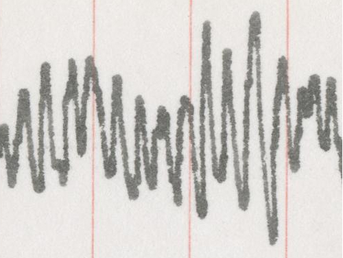
I chose a starting segment to work on that represents a good section of data, with some overlap and high amplitude:

I first tried the method described in McKeown et al. (1997), which works pretty well except for cases where the width of the pen and curvature due to the tracing apparatus contaminate neighboring columns. This results in a few jumps/irregularities where the line should be smooth and some loss of amplitude:

Then I tried skeletonization using the built-in MATLAB image processing algorithm, which seems to better represent amplitude (see image below). Wang et al.'s paper describes a method for choosing one point per column by starting from the left and using the next closest possibility, but as suggested by Chris in class, I will look into a hybrid of these two overall methods and once in the time domain, use a low pass filter since I'm only interested in 8-13 Hz.

WEEK 6

Continuing from last week, I worked on refining both methods. For the first method, I improved the algorithm by choosing only contiguous sections of black pixels in each column, resulting in an improved selection of amplitude, but more noise. This will be filtered with a low pass once I convert to the time domain:

For the second method, skeletonizing, I averaged the amplitude in each column of pixels and the results are not too bad (see below). I will work on combining these methods, moving into the time domain, and alpha analysis next.

WEEK 7 - FINALIZED ALGORITHM / IMAGE REGISTRATION

This week I finalized my algorithm for reducing my image to a single pixel (or amplitude) per column of pixels; if the above 2 methods produce a value, average them, otherwise choose the one with a value. If neither method produced a value, set the pixel value to zero and perform cubic interpolation on any zeros at the end.

I also worked on a method to automatically chop off the left and right edges of the page, separate the upper and lower traces, and remove the line numbers. Using the image processing toolbox in MATLAB, I can align an image with a trace to a template image (blank page I found without any data). It works best if I remove the trace and align the portion of the image that will match. This will be possible for about half of the pages we have, as the rest have been cut off to include only the trace, and the alignment functions do not work well. For those, I have a manual pipeline, and perhaps with more time I can tweak the alignment functions to do this. Here is my template image:

WEEK 8 - CONVERSION TO TIME DOMAIN

Converting to the time domain involves determining the conversion factor for the xand y axes that moves from pixels to time or amplitude. For the x-axis, this is tricky as we have no indication on the data itself as to the recording speed. However, there is an indication in a document describing the setup of the EEG apparatus at UCSD, of either 10 seconds or 12 seconds per page. We will process the first few subjects at both speeds and see what we get in the alpha analysis. For the y-axis, many subjects have a reference section of the data with handwritten note for the amplitude value, but they are not consistent. Thus, we will normalize amplitude for the entire session for each subject.

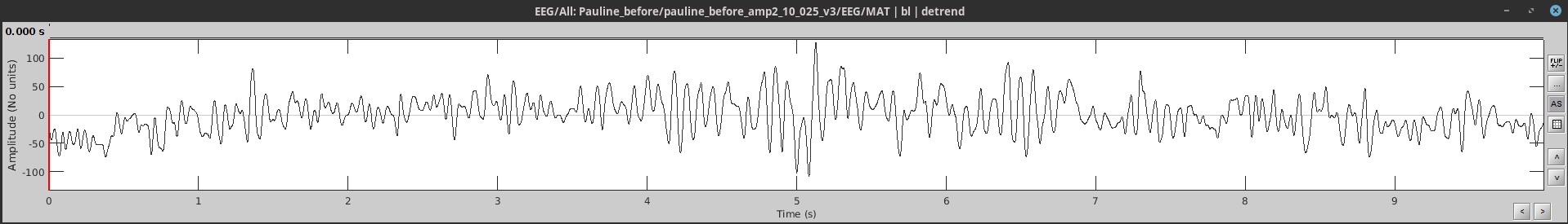
Here is an example of a time domain waveform. The x-axis is in milliseconds. Disregard the y-axis scale.

WEEK 9 - SPECTRAL ANALYSIS

This week I was able to work with the time domain waveform using the Brainstorm matlab toolbox for the processing that I am used to with EEG data, which means I can easily analyze spectral content to get a sense of alpha. Here's an example of the timeseries and time-frequency plot for one page:

WEEK 10 - PROCESSING PAULINE'S DATA

This last week I spent processing Pauline's 25 pages of before data in order to test out the full pipeline. However, I discovered that the image cleaning steps are incredibly time-consuming, and have decided to pause on full processing to try out a 3rd method of line extraction that may eradicate the need for all of the cleaning. The idea is to give a starting pixel on the left-most edge of the page in the middle of the trace. From there, move to the right and determine the average of the closest dark pixels. This allows for a tolerance within which to consider pixels because we know where exactly to start!

FUTURE

First to finalize will be the line extraction method and ways to minimize manual image cleaning. Then we can run all subjects' data through for before and after, as well as by condition. We'll need to determine most plausible recording speed, electrode locations, and look for any other trends.