 |
In Section 2.1.3, we discussed how digital waveguides model propagation of traveling waves
along a physical string. The single parameter that can change is the total delay in the loop.
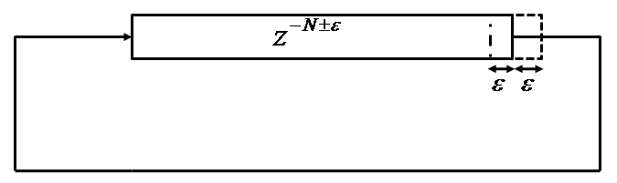
Since the described system is linear and time-invariant [3], the digital waveguide's delay lines, presented in
Section 2.1.3, can be lumped into one delay line with delay ![]() . Figure 16
shows such a simplification. Though this simplifies the block-diagram of a digital waveguide,
it loses its direct physical mapping: viewing the delay-lines as traveling waves moving in opposite directions.
However, the systems are equivalent. For our discussion on time-varying lengths for digital waveguides,
we discuss digital waveguide's with a single delay line, and thus with a single delay length.
. Figure 16
shows such a simplification. Though this simplifies the block-diagram of a digital waveguide,
it loses its direct physical mapping: viewing the delay-lines as traveling waves moving in opposite directions.
However, the systems are equivalent. For our discussion on time-varying lengths for digital waveguides,
we discuss digital waveguide's with a single delay line, and thus with a single delay length.
Once reduced to this form, the digital waveguide has a single parameter, its total delay ![]() . By changing
. By changing
![]() through time, the digital waveguide effectively models a changing propagation distance.
The most notable physical everyday occurrence of such an effect occurs whenever an ambulance or
police car with its sirens on passes us. The pitch of the siren increases on approach and decreases upon passing.
This phenomenon, known as the Doppler Effect [11], is the foundation behind many effects and sounds in the musical
community such as the flanger and the Leslie [12,13].
In the digital domain, however, changes in the delay line length
occurs in natural numbers. Fractions of samples in computers do not exist. Therefore,
in order to account for varying delay line lengths, many interpolation algorithms have been
studied to provide a smooth change in delay line lengths according to the sampling rate used
[14,15,16,17,18].
For a detailed overview of various interpolation methods, we refer the reader to
http://ccrma.stanford.edu/~jos/pasp/Delay_Line_Interpolation.html.
through time, the digital waveguide effectively models a changing propagation distance.
The most notable physical everyday occurrence of such an effect occurs whenever an ambulance or
police car with its sirens on passes us. The pitch of the siren increases on approach and decreases upon passing.
This phenomenon, known as the Doppler Effect [11], is the foundation behind many effects and sounds in the musical
community such as the flanger and the Leslie [12,13].
In the digital domain, however, changes in the delay line length
occurs in natural numbers. Fractions of samples in computers do not exist. Therefore,
in order to account for varying delay line lengths, many interpolation algorithms have been
studied to provide a smooth change in delay line lengths according to the sampling rate used
[14,15,16,17,18].
For a detailed overview of various interpolation methods, we refer the reader to
http://ccrma.stanford.edu/~jos/pasp/Delay_Line_Interpolation.html.
An online lab that steps the reader through digital implementations of the Doppler, Flanger and Leslie can be found at http://ccrma.stanford.edu/realsimple/doppler_flanger_leslie/.