The Octahedral Scheme

The grid for an octahedral scheme is constructed from two superimposed rectilinear grids; if the points of the first grid are located at cube corners, then the points of the second will occur at the centers of the cubes defined by the first. The relevant difference scheme on an octahedral grid can be written as

$$\begin{split}U_{i,j,k}(n+1)+U_{i,j,k}(n-1) &= \frac{3}{4}\lam... ...g)\\ &\quad+\left(2-8\lambda^{2}\right)U_{i,j,k}(n) \end{split}$$ (28)

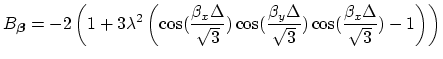
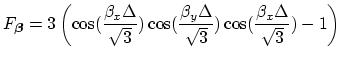
for $i$, $j$ and $k$ which are either all even or all odd integers. Now, we have taken the spacing between nearest neighbors to be $\Delta$, so the indices $i$, $j$ and $k$ refer to a point with coordinates $x=i\Delta/\sqrt{3}$, $y=j\Delta/\sqrt{3}$ and $z=k\Delta/\sqrt{3}$. The amplification polynomial equation is again of the form (5), with

$$B_{\mbox{{\scriptsize\boldmath$\beta$}}} = -2\left(1+3\lambda^{2}... ...eta_{y}\Delta}{\sqrt{3}})\cos(\frac{\beta_{x}\Delta}{\sqrt{3}})-1\right)\right)$$

and

$$F_{\mbox{{\scriptsize\boldmath$\beta$}}} = 3\left(\cos(\frac{\bet... ...frac{\beta_{y}\Delta}{\sqrt{3}})\cos(\frac{\beta_{x}\Delta}{\sqrt{3}})-1\right)$$

and it is again easy to determine that

$$\max_{\mbox{{\scriptsize\boldmath$\beta$}}}F_{\mbox{{\scriptsize\... ...ox{{\scriptsize\boldmath$\beta$}}}F_{\mbox{{\scriptsize\boldmath$\beta$}}} = -6$$

which are the same as the bounds in the cubic rectilinear case. We again have that

$$\lambda\leq\frac{1}{\!\!\sqrt{3}}$$

Thus the stability bound coincides with the passivity bound for the mesh implementation. For $\lambda = 1/\sqrt{3}$, instabilities may appear at any spatial frequency triplets $\beta$$= [\beta_{x}, \beta_{y}, \beta_{z}]^{T}$ where each component is either 0 or $\pm\sqrt{3}\pi/\Delta$.

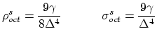
The computational and add densities are given by

$$\rho_{oct} = \frac{3\sqrt{3}v_{0}}{4\Delta^{4}}\hspace{0.5in}\sigma_{oct} = \frac{27\sqrt{3}v_{0}}{4\Delta^{4}}$$

for $v_{0}>\sqrt{3}\gamma$, and

$$\rho^{s}_{oct} = \frac{9\gamma}{8\Delta^{4}}\hspace{0.5in}\sigma^{s}_{oct} = \frac{9\gamma}{\Delta^{4}}$$

at the stability limit $v_{0} = \sqrt{3}\gamma$.

At the stability limit, the scheme can be divided into two mutually exclusive subschemes; plots of numerical dispersion are shown in Figure 9(b) and (c). It is interesting to note that there is no dispersion error along the six axial directions; this should be compared with the cubic rectilinear scheme, for which wave propagation is dispersionless along the diagonal directions (there are eight such directions).