Steven
Backer
sbacker @ ccrma
November
23, 2004
MUSIC 220A -
Foundations of Computer Generated Sound
CCRMA, Stanford University
My goal seemed simple: explore uses of so-called “1/f noise” to algorithmically generate sounds from scheme code. Taking the time to learn about two concepts relatively new to me – scheme and 1/f noise – was worthwhile and quite educational, albeit time consuming. At this point, I am pleased with the results of this experiment, though I think what I have created lies somewhere between noise and music – call it “interesting sound” if you will. This was certainly an academic exercise, rather than the creation of meaningful music. As one of my peers pointed out, one element that differentiates music from sound is meaning. (Perhaps this is what Pierce means about the creation of “highly artistic noise”.) Here, I will attempt to explain the processes I used, in hopes that the reader (and potential composer?) might gain an additional color for his/her compositional palette (probably of pinkish hue).
Background (on) Noise
Noise is just an audio signal represented by a sequence of random numbers. However, we can categorize different types of noisy sequences based on correlation within such a sequence. Many distinct, unique mathematical relationships can exist within a random sequence; Some commonly referred to types of noise are white noise, brown noise, and pink noise.
White noise (as an audio signal) has the property of containing the same amount of power across all frequencies. With true random numbers, there is zero correlation between successive samples of white noise. If you'd like to hear it, many sound clips of white noise can be found with Google, or you can create your own. The colored label “white” stems from the fact that white light contains an even distribution of wavelengths across the visible spectrum.
The Power Spectral Density (PSD) of a signal is a measure of the power of a signal over a range of time and frequencies. It can be thought of as the amount of power per unit frequency contained within a finite signal. There are many excellent resources available on the web explaining this in further detail (see below).
The PSD of white noise has a constant roll-off; that is, the slope of it's PSD remains constant as the PSD decreases across a linear range of frequencies. This could be thought of as proportional to 1/f0 (=1). Although the simplest to create, this noise is quite unnatural to our ears, which view the frequency domain on a logarithmic scale. Pink noise, on the other hand, is more natural to our ears, as it's PSD rolls off at a constant rate over frequencies heard on a logarithmic scale. On a linear scale, the PSD is seen to decrease at the rate of the inverse of it's frequency, or “1/f”. Brown noise is highly correlated, and has a PSD that rolls off at 1/f2. While white noise sequences are quite random, brown noise sequences are quite predictable over long periods of time. Pink noise lies somewhere in between.
If one were to create an audio signal in which the duration and frequency of successive notes were created by random numbers, the different “colors” of noise can be understood within a musical context. White noise sequences sound too random, and quite unmusical. Brown noise sequences sound too predictable, and musically uninteresting. Pink noise, however, often creates sequences perceived as musical – changes occur in a manner often perceived as “intelligent”.
Interestingly enough, patterns of 1/f fluctuations can be found in an enormous number of examples of real world phenomena. Some examples of 1/f fluctuations have been found in sunspot activity, nerve membranes, flood levels of the Nile river, electronic devices, the period of the heartbeat, traffic patterns, written language, work tardiness, DNA sequences, astronomy, and of course, MUSIC. Voss and Clark published a seminal paper in a 1978 issue of The Journal of the Acoustical Society of America which relates 1/f fluctuations to a variety of musical works. They show that many notable works have a PSD with a 1/f roll-off. Among those cited are Bach's First Brandenburg Concerto, Scott Joplin piano rags, a classical radio station, Davidovsky's Synchronism I, II, and III, Milton Babbit's String Quartet No. 3, a piano concerto by Elliot Carter, and Stockhausen's Momente. This stunning correlation of 1/f noise to many notable compositions suggests that highly musical sequences often contain 1/f fluctuations. Thus, there is much interest in using algorithms utilizing 1/f noise processes as a compositional tool, especially within computer generated music.
Creating Pink Noise
Creating perfect pink noise is an impossible task. We would need an infinite number of samples to ensure that an equal distribution of power per octave is contained in a signal all the way down to dc. However, it is possible to create a close approximation of pink noise over the audio band in a finite duration sequence. One popular method for generating 1/f noise is to filter white noise using a “pinking filter” characterized by having a filter gain that rolls of at 3-dB per octave in the frequency domain. Julius Smith has created a fine pinking filter, which is outlined in the references below.
To create 1/f noise for my sketch, I implemented Julius' pinking filter in matlab. My matlab code can be found here. I created three separate streams of pink noise, each of length N=120, which I then used to control various aspects of sound synthesis. This was accomplished by saving the random sequences from matlab in a text file, and then reading in these values from each file within my scheme code. More on this below.
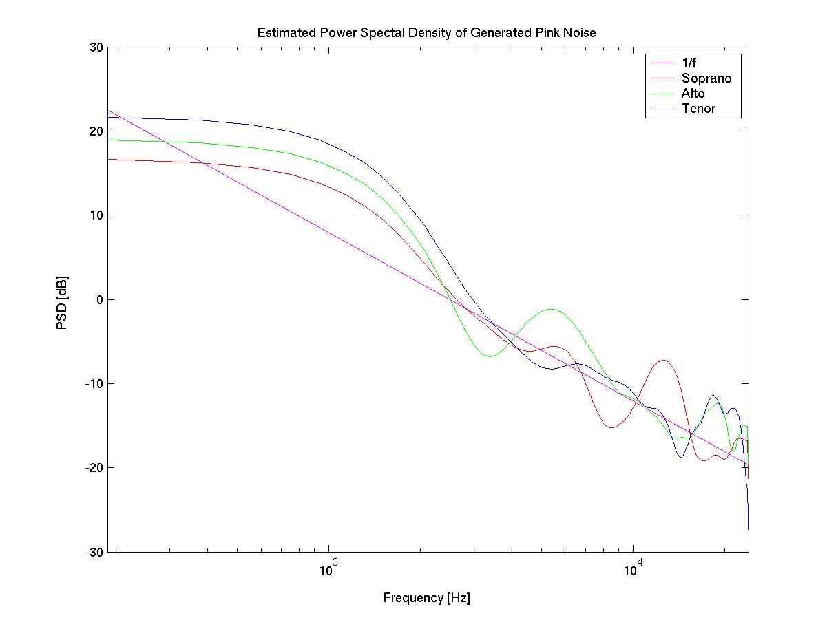
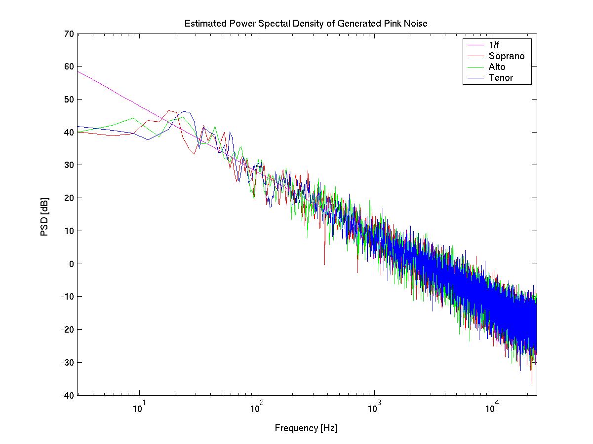
To ensure the noise I created was indeed pink (or at least close to pink), I also performed a rough analysis of the power spectral density of these sequences. The plot below shows the PSD for the three sequences (named Soprano, Alto, and Tenor), compared to the ideal 1/f trend. It can be seen that these sequences do indeed have a PSD that rolls off at approximately 1/f. Note that closer to DC, the trend begins to vary further from the ideal, as it gets more difficult to obtain the ideal distribution with such a limited number of samples. Also, the minimum frequency at which we can analyze the PSD is limited by the small number of samples. The second plot shows the performance of the filter with a much larger number of samples. This analysis encompasses most of the audio band, and clearly shows that the 1/f trend is created with high accuracy by this pinking filter.
PSD for the sequences I used in my sketch:
PSD for a large number of samples (for analysis only):
A Noisy Scheme Process
Rather than map pink noise directly to note values, I wanted to investigate the effects of using this noise to control other synthesis parameters such as amplitude, note duration, wait time between notes, and pitch detuning. I chose to specify all of the base note values explicitly, relinquishing little control over this matter to the computer. To do this, I used notes from some old four-part harmony I had lying around (ask me if you would like to see the original score). I stripped out all of the extra eighth notes, and simply entered in 4 sequences of 60 notes each into scheme corresponding to the quarter notes in my original counterpoint. At this point, the rules used to create the original harmony have been thrown out the window.
For the soprano, tenor, and alto voices, the 1/f sequences were used to control synthesis parameters, though quite indirectly. Scheme code reads in the random sequences via an input file stream. I have modified the random sequences as needed for implementation, so this should not be thought of as a direct mapping of 1/f noise, but rather a mapping that originates from the generation of such sequences. For example, it would not be appropriate to use negative values for note duration. Since negative values exist in the zero-mean sequence, I had to make changes in the sequence to ensure the values were permissible for synthesis.
The very same scheme code also creates a score for a human bass player. My goal was to keep this voice within a reasonable range of human performer capability (with regard to notation), thus I have not used 1/f noise in the bass voice. However, the computer generated accompaniment also subtly includes this voice. The advantage here is that the note sequence for the human performer can be simply altered within the scheme code, and the resulting accompaniment will also reflect such changes, in a very indirect manner, musically speaking. I chose use an arbitrary “bass” instrument since the bass (be it electric, double-bass, voice, or other) often takes on a supporting role in music. Victor Wooten recently said that the bass can be thought of as the cake that holds up the icing, making the overly sweet icing palatable in larger doses. By the end of my sketch, it seems as though the cake has been inverted, as the computer accompaniment shifts from being the primary focus to a more supportive role.
Here is the final scheme code:
(Note:
This implementation works as I intended it to,
but contains some
less-than-optimal coding due to my
limited understanding of scheme
and CLM.
While it is quite slow, it gets the job done!)
And the MIDI score for a human bass player:
Final mix of the accompaniment and the bass part (realized with a MIDI acoustic bass):
Selected References:
Clarke, J. and Voss, R. F., "1/f Noise in Music: Music from 1/f Noise," Journal of the Acoustical Society of America, 63(1), 1978, 258-263.
Smith,
Julius O. Introduction
to Digital Filters, May 2004 Draft,
Center for
Computer Research in Music and Acoustics (CCRMA), Stanford
University.
http://www.firstpr.com.au/dsp/pink-noise/
For fun, here are some extra sound clips made in the process of creating the work above:
I guess that the quite enjoyable 220a homework sequence is over...though I feel I was once told that the Moment Never Ends. Part of my inspiration for this assignment is Mike Gordon's bass playing – OUT front and in the lead, yet still supportive; somewhere between white and brown.