Fourier Transforms for Continuous/Discrete Time/Frequency

The Fourier transform can be defined for signals which are

• discrete or continuous in time, and
• finite or infinite in duration.

This results in four cases. As you might expect, the frequency domain has the same cases:

• discrete or continuous in frequency, and
• finite or infinite in bandwidth.

When time is discrete, the frequency axis is finite, and vice versa.

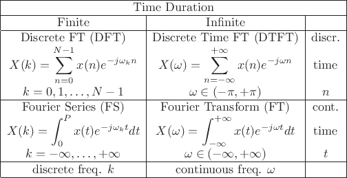
Reference [243] develops the DFT in detail--the discrete-time, discrete-frequency case. In the DFT, both the time and frequency axes are finite in length. Table 2.1 below summarizes the four Fourier-transform cases corresponding to discrete or continuous time and/or frequency. They are discussed further in [243].

Table 2.1: Four cases of sampled/continuous finite/infinite time and frequency.

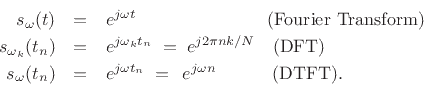
In all four cases, the Fourier transform can be interpreted as the inner product of the signal $x$ with a complex sinusoid at radian frequency $\omega$ [243]:

$$X(\omega) = \left<x,s_\omega\right>$$

where $s_\omega$ is appropriately adapted, e.g.,

• $e^{j\omega t}$ (Fourier transform case),
• $e^{j\omega n}$ (DTFT case),
• $e^{j2\pi k n/N}$ (DFT case).

In spectral modeling of audio, we usually deal with indefinitely long signals. Fourier analysis of an indefinitely long discrete-time signal is carried out using the Discrete Time Fourier Transform (DTFT). In practical situations we can only deal with finite-duration signals, so really we will always use the Discrete Fourier Transform (DFT) [243].

In the remainder of this chapter, the DTFT is defined and selected Fourier theorems are stated and proved for the DTFT case. Additionally, the Fourier Transform (FT) is defined, and selected FT theorems are stated and proved as well. The theorems for the DFT case are detailed in [243].