 |
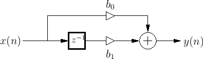
Figure B.1 gives the signal flow graph for the general one-zero filter. The frequency response for the one-zero filter may be found by the following steps:
![\fbox{
\begin{tabular}{rl}
Difference equation: & $y(n) = b_0x(n) + b_1x(n - 1)$\ \\ [5pt]
{\it z} transform: & $Y(z) = b_0X(z) + b_1z^{-1}X(z)$\\ [5pt]
Transfer function: & $H(z) = b_0 + b_1z^{-1}$\\ [5pt]
Frequency response: & $H(e^{j\omega T}) = b_0 + b_1e^{-j\omega T}$
\end{tabular}}](img1348.png)
By factoring out
![]() from the frequency response, to
balance the exponents of
from the frequency response, to
balance the exponents of ![]() , we can get this closer to polar form as
follows:
, we can get this closer to polar form as
follows:
 |
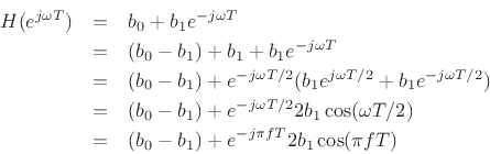
We now apply the general equations given in
Chapter 7 for filter gain ![]() and filter phase
and filter phase
![]() as a function of frequency:
as a function of frequency:
![\begin{eqnarray*}
H(e^{j\omega T}) &=& b_0 + b_1e^{-j\omega T}\\
&=& b_0 + b_1 \cos(\omega T) - jb_1 \sin(\omega T)\\ [10pt]
G(\omega) &=& \sqrt{[b_0 + b_1 \cos(\omega T)]^2 + [-b_1 \sin(\omega T)]^2}\\
&=& \sqrt{b_0^2 + b_1^2 + 2b_0b_1 \cos(\omega T)}\\ [10pt]
\Theta(\omega) &=& \tan^{-1}\left[\frac{-b_1 \sin(\omega T)}{b_0 + b_1 \cos(\omega T)}\right]
\end{eqnarray*}](img1352.png)
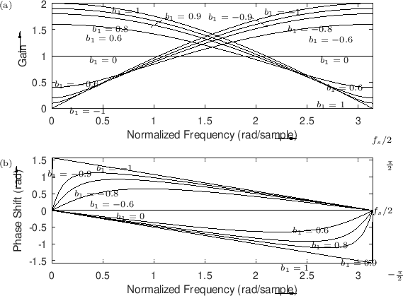
A plot of ![]() and
and
![]() for
for ![]() and various
real values of
and various
real values of ![]() , is given in Fig.B.2. The filter has a zero
at
, is given in Fig.B.2. The filter has a zero
at
![]() in the
in the ![]() plane, which is always on the
real axis. When a point on the unit circle comes close to the zero of
the transfer function the filter gain at that frequency is
low. Notice that one real zero can basically make either a highpass
(
plane, which is always on the
real axis. When a point on the unit circle comes close to the zero of
the transfer function the filter gain at that frequency is
low. Notice that one real zero can basically make either a highpass
(
![]() ) or a lowpass filter (
) or a lowpass filter (
![]() ). For the phase
response calculation using the graphical method, it is necessary to
include the pole at
). For the phase
response calculation using the graphical method, it is necessary to
include the pole at ![]() .
.