One-Pole

Figure B.3: Signal flow graph for the general one-pole filter

Fig.B.3 gives the signal flow graph for the general one-pole filter. The road to the frequency response goes as follows:

Figure B.4: Family of frequency responses of the one-pole filter

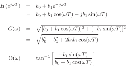
The one-pole filter has a transfer function (hence frequency response) which is the reciprocal of that of a one-zero. The analysis is thus quite analogous. The frequency response in polar form is given by

$$\begin{eqnarray*} G(\omega) &=& \frac{\vert b_0\vert}{\sqrt{[1 + a_1 \cos(\omega T)]^2 + [-a_1 \sin(\omega T)]^2}}\\ &=& \frac{\vert b_0\vert}{\sqrt{1 + a_1^2 + 2a_1 \cos(\omega T)}}\\ [10pt] \Theta(\omega) &=& \left\{\begin{array}{ll} -\tan^{-1}\left[\frac{-a_1 \sin(\omega T)}{1 + a_1 \cos(\omega T)}\right], & b_0>0 \\ [5pt] \pi-\tan^{-1}\left[\frac{-a_1 \sin(\omega T)}{1 + a_1 \cos(\omega T)}\right], & b_0<0 \\ \end{array} \right.. \end{eqnarray*}$$

A plot of the frequency response in polar form for $b_0 = 1$ and various values of $a_1$ is given in Fig.B.4.

The filter has a pole at $z = -a_1$ , in the $z$ plane (and a zero at $z$ = 0). Notice that the one-pole exhibits either a lowpass or a highpass frequency response, like the one-zero. The lowpass character occurs when the pole is near the point $z = 1$ (dc), which happens when $a_1$ approaches $-1$ . Conversely, the highpass nature occurs when $a_1$ is positive.

The one-pole filter section can achieve much more drastic differences between the gain at high frequencies and the gain at low frequencies than can the one-zero filter. This difference is achieved in the one-pole by gain boost in the passband rather than attenuation in the stopband; thus it is usually desirable when using a one-pole filter to set $b_0$ to a small value, such as $1 - \left\vert a_1\right\vert$ , so that the peak gain is 1 or so. When the peak gain is 1, the filter is unlikely to overflow.^B.1

Finally, note that the one-pole filter is stable if and only if $\left\vert a_1\right\vert < 1$ .