In this example, we consider a second-order filter (![]() ) with two
inputs (
) with two
inputs (![]() ) and two outputs (
) and two outputs (![]() ):
):
![\begin{eqnarray*}
A &=& g\left[\begin{array}{rr} c & -s \\ [2pt] s & c \end{array}\right]\quad \mbox{with $c^2+s^2=1$\ and $0<g<1$}\\ [10pt]
B &=& \left[\begin{array}{cc} 1 & 0 \\ [2pt] 0 & 1 \end{array}\right]\qquad
C = \left[\begin{array}{cc} 1 & 0 \\ [2pt] 0 & 1 \end{array}\right]\qquad
D = \left[\begin{array}{cc} 0 & 0 \\ [2pt] 0 & 0 \end{array}\right]
\end{eqnarray*}](img2119.png)
so that
![\begin{eqnarray*}
\left[\begin{array}{c} x_1(n+1) \\ [2pt] x_2(n+1) \end{array}\right]
&=&
g\left[\begin{array}{rr} c & -s \\ [2pt] s & c \end{array}\right]
\left[\begin{array}{c} x_1(n) \\ [2pt] x_2(n) \end{array}\right]
+
\left[\begin{array}{cc} 1 & 0 \\ [2pt] 0 & 1 \end{array}\right]
\left[\begin{array}{c} u_1(n) \\ [2pt] u_2(n) \end{array}\right],\\ [10pt]
\left[\begin{array}{c} y_1(n) \\ [2pt] y_2(n) \end{array}\right]
&=&
\left[\begin{array}{cc} 1 & 0 \\ [2pt] 0 & 1 \end{array}\right]
\left[\begin{array}{c} x_1(n) \\ [2pt] x_2(n) \end{array}\right].
\end{eqnarray*}](img2120.png)
From Eq.(G.5), the transfer function of this MIMO digital filter is then
![\begin{eqnarray*}
H(z) &=& C(zI-A)^{-1}B = (zI-A)^{-1} = \left[\begin{array}{cc} z-gc & gs \\ [2pt] -gs & z-gc \end{array}\right]^{-1}\\ [5pt]
&=&\frac{1}{z^2-2gcz +g^2c^2+g^2s^2}\left[\begin{array}{cc} z-gc & -gs \\ [2pt] gs & z-gc \end{array}\right]\\ [5pt]
&=&\left[\begin{array}{cc} \frac{\displaystyle z^{-1}-gcz^{-2}}{\displaystyle 1-2gcz^{-1}+g^2z^{-2}} & -\frac{\displaystyle sz^{-2}}{\displaystyle 1-2gcz^{-1}+g^2z^{-2}} \\ [5pt] \frac{\displaystyle gsz^{-2}}{\displaystyle 1-2gcz^{-1}+g^2z^{-2}} & \frac{\displaystyle z^{-1}-gcz^{-2}}{\displaystyle 1-2gcz^{-1}+g^2z^{-2}} \end{array}\right].
\end{eqnarray*}](img2121.png)
Note that when ![]() , the state transition matrix
, the state transition matrix ![]() is simply a 2D
rotation matrix, rotating through the angle
is simply a 2D
rotation matrix, rotating through the angle ![]() for which
for which
![]() and
and
![]() . For
. For ![]() , we have a type of
normalized second-order resonator [51],
and
, we have a type of
normalized second-order resonator [51],
and ![]() controls the ``damping'' of the resonator, while
controls the ``damping'' of the resonator, while
![]() controls the resonance frequency
controls the resonance frequency ![]() . The resonator
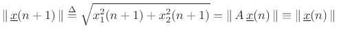
is ``normalized'' in the sense that the filter's state has a constant
. The resonator
is ``normalized'' in the sense that the filter's state has a constant
![]() norm (``preserves energy'') when
norm (``preserves energy'') when ![]() and the input is zero:
and the input is zero:
In this two-input, two-output digital filter, the input ![]() drives state
drives state ![]() while input
while input ![]() drives state
drives state ![]() .
Similarly, output
.
Similarly, output ![]() is
is ![]() , while
, while ![]() is
is ![]() .
The two-by-two transfer-function matrix
.
The two-by-two transfer-function matrix ![]() contains entries for
each combination of input and output. Note that all component
transfer functions have the same poles. This is a general property of
physical linear systems driven and observed at arbitrary points: the
resonant modes (poles) are always the same, but the zeros vary as the
input or output location are changed. If a pole is not visible using
a particular input/output pair, we say that the pole has been
``canceled'' by a zero associated with that input/output pair. In
control-theory terms, the pole is ``uncontrollable'' from that input,
or ``unobservable'' from that output, or both.
contains entries for
each combination of input and output. Note that all component
transfer functions have the same poles. This is a general property of
physical linear systems driven and observed at arbitrary points: the
resonant modes (poles) are always the same, but the zeros vary as the
input or output location are changed. If a pole is not visible using
a particular input/output pair, we say that the pole has been
``canceled'' by a zero associated with that input/output pair. In
control-theory terms, the pole is ``uncontrollable'' from that input,
or ``unobservable'' from that output, or both.